Download
1 / 46
460 likes | 596 Views
CSE 554 Lecture 6: Fairing and Simplification. Fall 2012. Review. Iso-contours in grayscale images and volumes Piece-wise linear representations Polylines (2D) and meshes (3D) Primal and dual methods Marching Squares (2D) and Cubes (3D) Dual Contouring (2D,3D)

E N D
Review • Iso-contours in grayscale images and volumes • Piece-wise linear representations • Polylines (2D) and meshes (3D) • Primal and dual methods • Marching Squares (2D) and Cubes (3D) • Dual Contouring (2D,3D) • Acceleration using trees • Quadtree (2D), Octree (3D) • Interval trees
Geometry Processing • Fairing (smoothing) • Relocating vertices to achieve a smoother appearance • Simplification • Reducing vertex count • Deformation • Relocating vertices guided by user interaction or to fit onto a target
Points and Vectors • Same representation • Different meaning: • Point: a fixed location (relative to {0,0} or {0,0,0}) • Vector: a direction and magnitude • No location (any location is possible) Y 2 x 1 2
Point Operations • Subtraction • Result is a vector • Addition with a vector • Result is a point • Can points add? • Not yet…
Vector Operations • Addition/Subtraction • Result is a vector • Scaling by a scalar • Result is a vector • Magnitude • Result is a scalar • A unit vector: • To make a unit vector (normalization):
Adding Points • Affine combinations • Weighted addition of points where all weights sum to 1 • Result is another point • Same as adding scaled vectors to a point
Adding Points • Affine combinations: examples • Mid-point of two points • Linear interpolation of two points • Centroid of multiple points
Geometry Processing • Fairing (smoothing) • Relocating vertices to achieve a smoother appearance • Simplification • Reducing vertex count
Fairing (2D) • Reducing “bumpiness” by changing the vertex locations
Fairing (2D) • What is a bump? • A vertex far from the mid-point of its two neighbors A big bump A small bump
Fairing (2D) • Fairing by mid-point averaging • Moving each vertex towards the mid-point of its two neighbors • Using linear interpolation • : some value between 0 and 1 • Controls how far p’ moves away from p • Iterative fairing • At each iteration, update all vertices using locations in the previous iteration • A close to 1 will create oscillation • Typically
Fairing (2D) • Drawback • The initial shape is shrunk! 100 iterations 200 iterations 400 iterations
Fairing (2D) • Non-shrinking mid-point averaging [Taubin 1995] • Alternate between two kinds of iterations with different • Odd iterations: (positive) • Shrinking the shape • Even iterations: (negative) • : typically 0.1 • Expanding the shape
Fairing (2D) • The initial shape is no longer shrunk • The result converges with increasing iterations 100 iterations 200 iterations 400 iterations
Fairing (3D) • Fairing by centroid averaging • Moving each vertex towards the centroid of its edge-adjacent neighbors (called the 1-ring neighbors) • Linear interpolation • Iterative, non-shrinking fairing • Alternate between shrinking and expanding • Same choices of as in 2D • Each iteration updates all vertices using locations in the previous iteration centroid
Fairing (3D) • Example: fairing iso-surface of a binary volume
Fairing • Implementation Tips • At each iteration, keep two copies of locations of all vertices • Store the smoothed location of each vertex in another list separate from the current locations • Building an adjacency table storing the neighbors of each vertex would be helpful, but not necessary • Initialize the centroid as {0,0,0} at each vertex, and its neighbor count as 0. • For each triangle, add the coordinates of each vertex to the centroids stored at the other two vertices and increment their neighbor count. • The neighbor count is twice the actual # of edge neighbors • For each vertex, divide the centroid by its neighbor count.
More Vector Operations • Dot product (in both 2D and 3D) • Result is a scalar • In coordinates (simple!) • 2D: • 3D: • Matrix product between a row and a column vector
h More Vector Operations • Uses of dot products • Angle between vectors: • Orthogonal: • Projected length of onto :
More Vector Operations • Cross product (only in 3D) • Result is another 3D vector • Direction: Normal to the plane where both vectors lie (right-hand rule) • Magnitude: • In coordinates:
More Vector Operations • Uses of cross products • Getting the normal vector of the plane • E.g., the normal of a triangle formed by • Computing area of the triangle formed by • Testing if vectors are parallel:
More Vector Operations (Sign change!)
Geometry Processing • Fairing (smoothing) • Relocating vertices to achieve a smoother appearance • Simplification • Reducing vertex count
Simplification (2D) • Representing the shape with fewer vertices (and edges) 200 vertices 50 vertices
Simplification (2D) • If I want to replace two vertices with one, where should it be?
After replacement: Simplification (2D) • If I want to replace two vertices with one, where should it be? • Shortest distances to the supporting lines of involved edges
Simplification (2D) • Distance to a line • Line represented as a point q on the line, and a perpendicular unit vector (the normal) n • To get n: take a vector {x,y} along the line, n is {-y,x} followed by normalization • Distance from any point p to the line: • Projection of vector (p-q) onto n • This distance has a sign • “Above” or “under” of the line • We will use the distance squared Line
Simplification (2D) • Closed point to multiple lines • Sum of squared distances from p to all lines (Quadratic Error Metric, QEM) • Input lines: • We want to find the p with the minimum QEM • Since QEM is a convexquadratic function of p, the minimizing p is where the derivative of QEM is zero, which is a linear equation
Row vector Matrix transpose [Eq. 1] Matrix (dot) product 2x2 matrix 1x2 column vector Scalar Simplification (2D) • Minimizing QEM • Writing QEM in matrix form
Simplification (2D) • Minimizing QEM • Solving the zero-derivative equation: • A linear system with 2 equations and 2 unknowns (px,py) • Using Gaussian elimination, or matrix inversion: [Eq. 2]
Simplification (2D) • What vertices to merge first? • Pick the ones that lie on “flat” regions, or whose replacing vertex introduces least QEM error.
Simplification (2D) • The algorithm • Step 1: For each edge, compute the best vertex location to replace that edge, and the QEM at that location. • Store that location (called minimizer) and its QEM with the edge.
Simplification (2D) • The algorithm • Step 1: For each edge, compute the best vertex location to replace that edge, and the QEM at that location. • Store that location (called minimizer) and its QEM with the edge. • Step 2: Pick the edge with the lowest QEM and collapse it to its minimizer. • Update the minimizers and QEMs of the re-connected edges.
Simplification (2D) • The algorithm • Step 1: For each edge, compute the best vertex location to replace that edge, and the QEM at that location. • Store that location (called minimizer) and its QEM with the edge. • Step 2: Pick the edge with the lowest QEM and collapse it to its minimizer. • Update the minimizers and QEMs of the re-connected edges.
Simplification (2D) • The algorithm • Step 1: For each edge, compute the best vertex location to replace that edge, and the QEM at that location. • Store that location (called minimizer) and its QEM with the edge. • Step 2: Pick the edge with the lowest QEM and collapse it to its minimizer. • Update the minimizers and QEMs of the re-connected edges. • Step 3: Repeat step 2, until a desired number of vertices is left.
Simplification (2D) • The algorithm • Step 1: For each edge, compute the best vertex location to replace that edge, and the QEM at that location. • Store that location (called minimizer) and its QEM with the edge. • Step 2: Pick the edge with the lowest QEM and collapse it to its minimizer. • Update the minimizers and QEMs of the re-connected edges. • Step 3: Repeat step 2, until a desired number of vertices is left.
Simplification (2D) • Step 1: Computing minimizer and QEM on an edge • Consider supporting lines of this edge and adjacent edges • Compute and store at the edge: • The minimizing location p (Eq. 2) • QEM (substitute p into Eq. 1) • Used for edge selection in Step 2 • QEM coefficients (a, b, c) • Used for fast update in Step 2 Stored at the edge:
Simplification (2D) • Step 2: Collapsing an edge • Remove the edge and its vertices • Re-connect two neighbor edges to the minimizer of the removed edge • For each re-connected edge: • Increment its coefficients by that of the removed edge • The coefficients are additive! • Re-compute its minimizer and QEM Collapse : new minimizer locations computed from the updated coefficients
Simplification (3D) • The algorithm is similar to 2D • Replace two edge-adjacent vertices by one vertex • Placing new vertices closest to supporting planes of adjacent triangles • Prioritize collapses based on QEM
Simplification (3D) • Distance to a plane (similar to the line case) • Plane represented as a point q on the plane, and a unit normal vector n • For a triangle: n is the cross-product of two edge vectors • Distance from any point p to the plane: • Projection of vector (p-q) onto n • This distance has a sign • “above” or “below” the plane • We use its square
3x3 matrix 1x3 column vector Scalar Simplification (3D) • Closest point to multiple planes • Input planes: • QEM (same as in 2D) • In matrix form: • Find p that minimizes QEM: • A linear system with 3 equations and 3 unknowns (px,py,pz)
Simplification (3D) • Step 1: Computing minimizer and QEM on an edge • Consider supporting planes of all triangles adjacent to the edge • Compute and store at the edge: • The minimizing location p • QEM[p] • QEM coefficients (a, b, c) The supporting planes for all shaded triangles should be considered when computing the minimizer of the middle edge.
Simplification (3D) Degenerate triangles after collapse • Step 2: Collapsing an edge • Remove the edge with least QEM • Re-connect neighbor triangles and edges to the minimizer of the removed edge • Remove “degenerate” triangles • Remove “duplicate” edges • For each re-connected edge: • Increment its coefficients by that of the removed edge • Re-compute its minimizer and QEM Duplicate edges after collapse Collapse
Simplification (3D) • Example: 5600 vertices 500 vertices
Further Readings • Fairing: • “A signal processing approach to fair surface design”, by G. Taubin (1995) • No-shrinking centroid-averaging • Google citations > 1000 • Simplification: • “Surface simplification using quadric error metrics”, by M. Garland and P. Heckbert (1997) • Edge-collapse simplification • Google citations > 2000