Download
1 / 42
420 likes | 539 Views
Local Polynomial Method for Ensemble Forecast of Time Series. Satish Kumar Regonda, Balaji Rajagopalan, Upmanu Lall, Martyn Clark, and Young-II Moon Hydrology Days 2005 Colorado State University, Fort Collins, CO. Time series modeling. Stochastic models (AR, ARMA,………)

E N D
Local Polynomial Method for Ensemble Forecast of Time Series Satish Kumar Regonda, Balaji Rajagopalan, Upmanu Lall, Martyn Clark, and Young-II Moon Hydrology Days 2005 Colorado State University, Fort Collins, CO
Time series modeling • Stochastic models (AR, ARMA,………) • Presume time series of a response variable as a realization of a random process xt=f(xt-1,xt-2,….xt-k) + et • Noise, finite data length, high temporal and spatial variation of the data influences estimation of “k” • Randomness in the system limits the predictability which could be • A result of many independent and irreducible degrees of freedom • Due to deterministic chaos
What is deterministic Chaos? Lorenz Attractor • Three coupled non-linear differential equations • System apparently seems erratic, complex, and almost random (and that are very sensitive to initial conditions), infact, the system is deterministic.
Chaotic systems Logistic Equation: Xn+1 =A* Xn*(1-Xn) ‘A’ is constant ‘Xn’ is Current Value ‘Xn+1’ is Future Value How these will be predicted? - “nonlinear dynamical based time series analysis”
Nonlinear Dynamics Based Forecasting procedure • xt= x1,x2,x3,…,xn • State space reconstruction (or dynamics recovery) using ‘m’ and ‘’ • Forecast for T time steps into future i.e., xt+T = f (Xt) + t • Xt is a feature vector • f is a linear or nonlinear function m = 3 and = 2
Local Map f • Forecast for ‘T’ time step into the future xt+T = f (Xt) + t • Typically, f(.) estimated locally within neighborhood of the feature vector • f (.) approximated using locally weighted polynomials defined as LOCFIT • Polynomial order ‘p’ • Number of neighbors K ( = *n, is fraction between (0,1] )
Estimation of m and tau.. • M is estimated using correlation dimension (Grassberger and Procaccio..xx) or False Neighbors (Kennel…xx) • Tau is estimated via Mutual Information (Sweeney, xx; Moon et al., 19xx)
Need for Ensembles.. • In real data, due to Noise (sampling and dynamical) the phase space parameters (i.e., Embedding dimension and Delay time) are not uniquely estimated. • Hence, a suite of plausible parameters of the state space i.e. D, , , p.
Cont’d • Forecast for ‘T’ time step into the future xt+T = f (Xt) + t • Typically, f(.) estimated locally within neighborhood of the feature vector • f (.) approximated using locally weighted polynomials defined as LOCFIT • Polynomial order ‘p’ • Number of neighbors K ( = *n, is fraction between (0,1] )
Cont’d • General Cross Validation (GCV) is used to select the optimal parameters ( and p) • Optimal parameter is the one that produces minimum GCV ei is the error n-number of data points m-number of parameters
Forecast algorithm • Compute D and using the standard methods and choose a broad range of D and values. • Reconstruct phase space for selected parameters • Calculate GCV for the reconstructed phase space by varying smoothening parameters of LOCFIT • Repeat steps 2 and 3 for all combinations of D, , , p • Select a suite of “best” parameter combinations that are within 5 percent of the lowest GCV • Each selected best combination is then used to generate a forecast.
Applications • Synthetic data • The Henon system • The Lorenz system • Geophysical data • The Great Salt Lake (GSL) • NINO3
Time series Henon X- ordinate Lorenz X- ordinate NINO3 GSL
Synthetic Data • The Lorenz system • A time series of 6000 observations generated • Embedding dimension: 2.06 and 3.0 • Training period: 5500 observations • Selected parameters: D = 2 & 3, = 1 & 2, and, p = 2 with various neighbor sizes (). • Forecasted 100 time steps into the future. • Predictability less than the Henon system ( large lyapunov exponent)
Blind Prediction Index 5368 Index 5371 Unstable Region Stable Region ~ 3 to 5 time steps ~ 35 points
The Great Salt Lake of Utah (GSL) • It is the fourth largest, perennial, closed basin, saline lake in the world. • Biweekly observations 1847-2002. • Superposition of strong and recurrent climate patterns at different timescales created a tough job of prediction for classical time series models. • Closed basin-----integrates hydrologic response and filters out high-frequency phenomenon and results into low dimensional phenomena. • GSL – is a low dimensional chaotic system (Sangoyomi et al. 1996)
GSL Attractor • Annual cycle is approximately motion around the smaller radius of the ‘spool’ • Longer term motion which has larger amplitude moves the orbits along the longer axis of the ‘spool’
Results • Embedding dimension: 4 ; delay time: 14 • GCV values computed over D = 2 to 6 and = 10 to 20, and p = 1 to 2, with various neighbor sizes • Fall of the lake volume • D = 4 & 5, = 10,14, &15, p = 1 &2, = 0.1-0.5 • Rise of the lake volume • D = 4 & 5, = 10 &15, p = 2, = 0.1-0.4
Blind Prediction Fall of the lake volume
Blind Prediction Rise of the lake volume
NINO3 • Time series of averaged monthly SST anomalies in the tropical Pacific covering the domain of 4oN-4oS and 90o-150oW • Monthly observations from 1856 onwards • ENSO characteristics (e.g. onset, termination, cyclic nature, partial locking to seasonal cycle, and irregularity) explained presuming system as low order chaotic system (embedding dimension 3.5; Tziperman et al. 1994 and 1995)
Results • El Nino Events (1982 and 1997): • 1982-83: D = 4 and = 16 • 1997-98: D = 5 and = 13 • Selected parameters range: D = 2 to 5, = 11 to 21 ( 8 to 16), p = 1& 2, = 0.1 – 1.0 • Forecasted issued in different months of the event • Ensemble prediction did a slightly better job compared to best AR-model
Blind Prediction 1997-98 El Nino
Results • La Nina events (1984 and 1989 ) • Both events yielded a dimension and delay time of 5 and 17 respectively. • Selected parameters range: D = 2 to 5, = 12 to 22, p = 1& 2, = 0.1 – 1.0 • Forecasted issued in different months • Both, ensemble and AR, methods performed similarly with increasing skill of the predictions when issued closer to the negative peak of the events
Blind Prediction 1999-2000 La Nina
Recent prediction May 1, 2002 July, 2004 (GSL) (NINO3)
Summary • A new algorithm proposed which selects a suite of ‘best’ parameters that captures effectively dynamics of the system • Ensemble forecasts provide • A natural estimate of the forecast uncertainty • The pdf of the response variable and consequently threshold exceedance probabilities • Decision makers will be benefited as forecast issued with a good lead-time • Performs better than the best AR-model • It could be improved in several ways
Acknowledgements • Thanks to CADSWES at the Univ. of Colorado at Boulder for letting use of its’ computational facilities. • Support from NOAA grant NA17RJ1229 and NSF grant EAR 9973125 are thankfully acknowledged.
Publication: - Regonda, S., B. Rajagopalan, U. Lall, M. Clark and Y. Moon, Local polynomial method for ensemble forecast of time series, (in press) Nonlinear Processes in Geophysics, Special issue on "Nonlinear Deterministic Dynamics in Hydrologic Systems: Present Activities and Future Challenges", 2005. Thank You
Lorenz attractor derived from a simplified model of convection to see the effect of initial conditions. The system is most commonly expressed as 3 coupled non-linear differential equations, which are known as Lorenz Equations. Lorenz Equations: dx / dt = a (y - x) dy / dt = x (b - z) - y dz / dt = xy - c z a, b, and c are the constants
Chua Attractor (electronic circuit) Duffing (nonlinear Oscillator)
State space reconstruction • Time series of observations xt= x1,x2,x3,………,xn • Embedding time series into ‘m’ dimensional phase space i.e., recovering dynamics of the system Xt = {xt, xt+, xt+ 2,…., xt+(m-1) } (Takens, 1981) m – embedding dimension - Delay time
Henon Lorenz D=2, Tau=1 Lorenz D=3, Tau=1 Lorenz D=3
Does GSL show Chaotic nature? • Long term persistence of the climate variations i.e., • because of superposition of strong, recurrent patterns at different scales makes difficult to justify classical, time series models • Closed basin-----integrates hydrologic response and filters out high-frequency phenomenon and results into low dimensional phenomena. • GSL – is a low dimensional chaotic system (Sangoyomi et al. 1996)
Blind Prediction 1982-83 El Nino
Blind Prediction 1984-85 La Nina
Nonlinear dynamics Based Time Series • State space reconstruction (Takens’ embedding theorem) Time series of a variable xt= x1,x2,x3,………,xn Xt = {xt, xt+, xt+ 2,…., xt+(m-1) } m – embedding dimension - Delay time 2. Fit a function that maps different states in the phase space
Cont’d Importance of ‘m’ and ‘’ U. Lalll, 1994
Chaotic behavior in geophysical processes • Lower order chaotic behavior observed in various geophysical variables (e.g., rainfall, runoff, lake volume) on different scales • Diagnostic tools • Grassberger-Procaccia algorithm • False Nearest Neighbors • Lyapunov Exponent
Results • The Henon system • 4000 observations of x-ordinate • Embedding dimension 2 and delay time 1 • Training period: 3700 observations and searched over D = 1 to 5 and = 1 to 10. • Selected combinations resulted 15 combinations and parameter values D = 2, = 1, p=2 and with various neighborhood sizes (i.e. ) • Forecasted 100 time steps into future
Blind prediction Index 3701 Index 3711 Ensemble forecast (5th&95th; 25th & 75th percentiles); Real observations; the best AR forecast