Download
1 / 37
400 likes | 627 Views
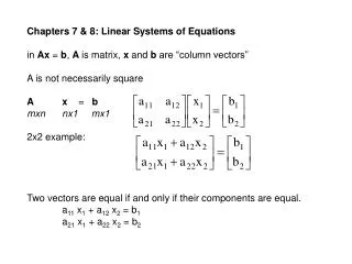
Chapters 7 & 8: Linear Systems of Equations in Ax = b , A is matrix, x and b are “column vectors” A is not necessarily square A x = b mxn nx1 mx1 2x2 example: Two vectors are equal if and only if their components are equal. a 11 x 1 + a 12 x 2 = b 1

E N D
Chapters 7 & 8: Linear Systems of Equations in Ax = b, A is matrix, x and b are “column vectors” A is not necessarily square A x = b mxn nx1 mx1 2x2 example: Two vectors are equal if and only if their components are equal. a11 x1 + a12 x2 = b1 a21 x1 + a22 x2 = b2
A solution of equation Ax = b can be thought of as a set of coefficients that defines a linear combination of the columns of A which equals column vector b. There may be no such set, a unique set, or multiple sets of the coefficients. If any set exist, then Ax = b is said to by “consistent”. If A is “non singular” then there exist A-1 such that A-1A = I then the unique solution is A-1A x = A-1b x = A-1b Explicit calculation of A-1is not an efficient method to solve linear equations. 1st objective: efficient solution when A is a square matrix. 2nd objective: meaning Ax = b when A is not square (discussed in the context of linear least squares problem)
Existence and Uniqueness: nxn matix A is nonsingular if any one of the following is true: (1) A has an inverse (2) det(A) 0 (3) rank(A) = n (rank = max number linearly independent rows or columns) (4) for any z0, A z0 If A-1 exist then x = A-1b is the unique solution of A x = b. If A is singular then, depending on b, one of the following is true: (1) no solution exist (inconsistent), (2) infinitely many solutions exist (consistent) A is singular and Ax = b has a solution, then there must be a z0 such that A z = 0 Then A (x + gz) = b and x + gz is a solution for any scalar g.
Span of a matrix span(A) defined as set of all vectors that can be formed by linear combinations of the columns of A. For nxn matrix, span(A) = { A x: x Rn } if A is singular and A x = b is inconsistent, then b span(A). if A is singular and A x = b is consistent, then b span(A).
Vector Norms: If p is a positive integer and x is an n-vector, then it p-norm is ||x||p = ( |xk|p)1/p Most commonly used p-norms are 1-norm ||x||1 = |xk| 2-norm ||x||2 = ( |xk|2)1/2 (Euclidean norm) -norm ||x|| = max1<k<n |xk|
Properties of all vector p-norms: ||x|| > 0 if x 0 ||gx|| > |g| ||x|| for any scalar g ||x + y|| < ||x|| + ||y|| (triangle inequality) | ||x|| - ||y|| | < ||x - y||
Matrix norms: ||A|| = maximum for all x 0 of Matrix norm defined this way said to be induced by or subordinate to the vector norm. Intuitively measures the maximum stretching that A does to any vector x.
Matrix norms that are easy to calculate: ||A||1 = maximum absolute column sum ||A|| = maximum absolute row sum ||A||1 is analogous to 1-norm of column vector ||A|| is analogous to -norm of column vector No analogy to vector Euclidean norm than can be easily calculated.
Properties of matrix norms: ||A|| > 0 if AO ||gA|| = |g| ||A|| for any scalar g ||A|| = 0 if and only if A = O. ||A + B|| < ||A|| + ||B|| ||A B|| < ||A|| ||B|| Special case: ||A x|| < ||A|| ||x|| for any column vector x
Sensitivity of the solution of Ax = b to input error E is error in A Db is error in b Dx is resulting error in solution ] < cond(A) [ + where cond(A) = ||A|| ||A-1||
Estimating cond(A): Singular value decomposition of A = USVT • is diagonal with elements sk that are the “singular values of A” Define Euclidean conditioning number cond2(A) = smax/smin If A is singular smin = 0 Determinant of A less than typical element of A
Residuals as a measure of the quality of an approximate solution: • Let x be an approximate solution to A x = b • Define residual r = b – Ax • ||Dx|| = ||x-x|| = ||A-1Ax – A-1b|| = ||A-1(Ax-b)|| = ||A-1r|| < ||A-1|| ||r|| • Divide by ||x||, introduce cond(A), and recall ||b|| < ||A|| ||x|| • Then <cond(A) <cond(A) • In an ill-conditioned problem (cond(A) >> 1) small residuals do not • imply a small error in an approximate solution
Solving Linear Systems: General strategy is to transform Ax = b in a way that does not effect the solution but renders it easier to calculate. Let M by any nonsingular matrix and z be the solution of M A z = M b Then z = (MA)-1Mb = A-1M-1M b = A-1b = x Call “premultiplying” or “multiply from the left” by M. Premultiplying by a nonsingular matrix does not change solution By repeated use of this fact Ax = b can be reduced to a “triangular” system
Triangular Linear Systems: In general, A in A x = b is “triangular” if it enables solution by successive substitution. Permutation of rows or columns allows a general triangular matrix to take the upper triangular form defined by (ajk = 0 if j > k) or the lower triangular form defined by (ajk = 0 if j < k) . If A is a upper triangular matrix, solve A x = b by backward substitution (pseudo-code p252 CK6) If A is a lower triangular matrix, solve A x = b by forward substitution x1 = b1/a11 xj = (bj - )/ajj j = 2,3, ...,n
Solution of Ax = b by Gaussian Elimination: Gaussian elimination (naïve or with pivoting) uses elementary elimination matricesto find matrix M such that MAx= Mb is an upper triangular system.
mj (j < k)=0 and mj (j > k) = aj/ak Mk = I – mekTek is kth column of I outer product nx1 times 1xn
Reduction of linear system Ax=b to upper triangular form Assume a11 is not zero Use a11 as pivot to obtain elementary elimination matrix M1 Multiply both sides of Ax=b by M1 (solution is unchanged) New system, M1Ax=M1b has zeroes in the 1st column except for a11 Assume a22 in M1A is not zero and use as pivot for M2 New system M2M1Ax=M2M1b has zeroes in the 1st and 2nd columns except for a11, a12, and a22 Continue until MAx=Mb, where M=Mn-1…M2M1 MA = U is upper triangular
LU factorization: Let L = M-1 = M1-1M2-1…Mn-1-1 Then LU = LMA =M-1MA = A A = LU called “LU factorization of A” Show that Lk = Mk-1 = I + mekT Proof: Mk-1Mk = (I+mekT)(I-mekT) = I – mekT + mekT + m(ekTm)ekT = I (ekTm) is a scalar = zero because only the non-zero component of ekT is ak and mk is zero.
Construction of L L = M-1 = M1-1M2-1…Mn-1-1 Note: order of Mk-1 in the product increases from left to right Mk-1Mj-1 = (I+mkekT)(I+mjejT) = I + mkekT + mjejT + mk (ekTmj )ejT (ekTmj ) is a scalar = 0 because the only non-zero component of ekT is ak and mj is zero if k < j Mk-1Mj-1 = I + mkekT + mjejT L = M-1 = M1-1M2-1…Mn-1-1 = I + m1e1T + … + mn-1en-1T L = identity matrix plus all the elementary elimination matrices used in the reduction of A to upper triangular form
Solving Ax =b by LU factorization of A Given L and U, how do we find x? Ux = MAx = Mb = y Multiply from left by L LUx = Ly Note that A = LU Ax = Ly Note that Ax = b b = Ly solve for y by forward substitution Given y, solve Ux = y by back substitution
Solving Ax =b using [eLt,U,P]=lu(A) P is the permutation matrix required to make PL explicitly lower triangular, eLt, which is form returned by MatLab Ux=MPAx=MPb= y Multiply from left by eLt eLtUx = eLty Note that PA = eLtU PAx = eLty Note that PAx=Pb Pb = eLtysolved for y by forward substitution Given y, solve Ux = y for x by back substitution
Gauss-Jordan and LU factorization are O(n3) G - J requires 3 times as many operations After A-1 calculated solution of Ax = b takes about the same number of n2 operations as LU factorization
Example of a rank-one update of A = If u=[1,0,0]T and v = [0,0,5]T then A – uvT =
vTA-1u is a scalar 1xn nxn nx1
Assignment 9, Due 4/8/14 Use the MATLAB function lu(A) to solve Ax = b where A = and b = Find the vectors u and v such that A’ = A – uvT differs from A by changing the sign of a12. Use the Sherman-Morrison method to solve A’y = b without refactoring. Write a MATLAB code for Cholesky factorization and use it to solve Ax = b by LU factorization when and b = A =
MatLab codes that you must write: . 1. backward substitution to solve A x = b if A is a upper triangular (see pseudo-code text p252) 2. forward substitution to solve A x = b if A is a lower triangular (see pseudo-code text p301 for a “unit” lower triangular) Forward substitution for non-unit lower triangular 3. Cholesky factorization to solve A x = b if A is positive definite (see pseudo-code text p305) x1 = b1/a11 xj = (bj - )/ajj j = 2,3, ...,n
Useful MatLab commands lu(A) LU factorization of A chol(A) Cholesky factorization of A A\b solves Ax = b condest(A) condition of A rcond(A) 1/condest(A) det(A) determinant of A
Chapter 7.1 Problems 7 p257 (use LU factorization) Computer problems 10, 11 p258 (use LU factorization) Chapter 7.2 Problems 1, 3 p272 Problems 2, 8, 9, 10 p 272-274 (use LU factorization) Computer problem 2, 3 p276 (use LU factorization) Chapter 8.1 Problems 1a, 2 p311 Problems 6d, 7 p312 (use your Cholesky factorization code) Problems 9b, 10, 11 p313 Computer problem 9b (use your Cholesky factorization code)