Download
1 / 70
700 likes | 713 Views
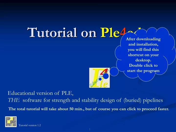
After downloading and installation, you will find this shortcut on your desktop. Double click to start the program. Tutorial on Ple 4 edu. Educational version of PLE, THE software for strength and stability design of (buried) pipelines.

E N D
After downloading and installation,you will find this shortcut on your desktop. Double click to start the program Tutorial on Ple4edu Educational version of PLE, THE software for strength and stability design of (buried) pipelines The total tutorial will take about 50 min., but of course you can click to proceed faster. Tutorial version 1.2 1
Some tips Use this presentation within Powerpoint 2003 or later because of the animations contained The presentation performs automatically and you can use the standard action buttons(down left). In case you want to skip screens, you can use the right mouse button. In case you want to pause the presentation, you may use as well the Pause/Break key on the keyboard (toggle). To open a table from an overview list, it is indicated as “Click”. This may be a ‘double click’ or a ‘single click+show button’ 2
Layout After clicking the shortcut the program will startup and will result in the following screen: Use this icon to show or hide the OVERVIEW panel Use this icon to show or hide the WORKSPACE panel Use this icon to show or hide the ROADMAP panel ..and if you are lost…use this icon to restore the default panel layout WORKSPACE panel OVERVIEW panel ROADMAP panel 3
Design function 1 Open new empty project We will now open a new ‘project’ and name it DEMO CASE Optional ‘project name’ Optional ‘project description’ …and ‘save’ Demo case 4
15 m Demo case Pipeline, crossing an old refilled ditch causing large soil settlements soil settlement Pipe Soil Pipeline bending stiffness partly resists deformation Questions: • To what extent will the pipeline follow the soil settlements? • What is the maximum stressing of the pipeline? 5
Limitations of educational version • General model only (no Code dependent features) • Maximum number of 50 elements (51 nodes) • No print or import/export options • No advanced options (branches, T-pieces, offshore, articulated, towing, material yielding, construction phasing etc) • But non-linear soil and geometrical behaviour included….. • and of course free use for educational purposes 6
construction subsidence 2 mm 500 mm main settlement area rigid, vertical roller support pipeline Elastically supported, half infinite pipeline connection soil Symmetry axis Modelling As a result of the limited availability of elements and the symmetry of the questions to be answered, the model will be cut at the mid settlement section, and at the other end far enough away from the settlement section to avoid interaction. 7
R1 R R2 M M1 C O construction subsidence 7300 2500 13500 100 100 100 elements 1. M at mid point 2. M1 near M to obtain near support internal forces 3. R at settlement transition 4. R1 and R2 near R for same reason 5. O at end of pipeline section considered 6. C at estimated point of maximum bending moment Symmetry axis Subdivision into elements main settlement area 1*100 15*487 2*100 5*500 27*500 total nr elements = 50 Main points 8
Global coordinate system Y-axis, horizontal and perpendicular to X-axis(right handed) Z-axis, perpendicularto X and Y axes, and pointing upward (right handed) X-axis here from M to O X-axis almost along pipeline ORIGIN 9
Click on the required ‘test’ icon to check the input data (if not yet available use the ‘more buttons’ facility) Click on the ‘default’ icon to get default ORIGIN-data (if not yet available use the ‘more buttons’ facility) Close table Design function 2 Now we will input the pipeline shape into the program. This is done in Design function 2 Click on DF2‘Pipeline Configuration’ Click on‘Pipeline origin’ Replace ‘start’ by ‘M’ 10
Point N Z(N) Point N+1 Z(N+1) R(N) line N Element length line N line N+1 Point N-1 DX(N) DX(N+1) Polygon Now the polygon has to be defined by means of the polygon points and their DX- and DY-distances relative to the previous point and their absolute Z-value. In this case all DY and Z-values remain zero. At the polygon points the radius of the pipe bend is provided.In this case there are no bends and this is specified by R = 0 The length of ‘pipe elements’ is specified per line between thepolygon point and the previous point. 11
R1 R R2 M M1 C O 7300 2500 13500 100 100 100 1*100 15*487 2*100 5*500 27*500 Test.. Symmetry axis Polygon table The table is rearranged a bit to fit all columns on the workspace. This can be done as well by hiding the roadmap. And the workspace is enlarged vertically Next we have to input the polygon points with lines attached ‘ENTER’ to get a new line click …and close next point …and so on 12
Locked tables & Set back All required data for this function has been provided and we will now process the function to be sure that indeed we do not exceed the allowable number of elements in this educational version Input tables are ‘locked’ because the results of this input are stored in the project database If you want to open the input tables again, click here to ‘set back’ the function. Results are removed from the project database in order to remain consistent. Click here to process the function 13
Check on node number Let’s have a look at the results of this function. For reason of clarity here the input tables list is hidden and the output tables list is made visible. Click here to maximize the workspace Click to see the ‘NODES’ list Check this box to show the output tables list Hide input tables list Scroll to end of table Indeed there are no more than 51 nodes. 14
Boundary conditions Boundary conditions DF 3.3 Pipe properties DF 3.1 Pipe/Soil properties DF 3.2 Eventually external supports The pipeline axis has been defined now and we proceed with specification of the pipe/soil properties in the Y-Z plane perpendicular to the pipeline axis Pipe axis DF = Design Function 15
Do WT Pipe data (DF3.1) • All data in N – mm - oC • Pipe material steelE = 2.1 105 N/mm2n = 0.3a = 12 10-6 mm/mm/oC • Pipe dimensionsDo = 1010 mmWT= 10 mm • Deadweight ignored 16
Material location table Click ‘Pipe data’ Click ‘material location’ Reference name of material to be specified X-coordinate where this material starts Test and Close 17
Isotropic material table Click ‘isotropic materials’ Shear modulus G is calculated from E and n, but can be overruled by an input datum Hide roadmap panel to free space for tables Use ‘test’ icon to see which data are ‘required’ Column headings speak for themselves Test and Close 18
Pipe diameter table Click ‘Outer diameter’ Procedure as before Test and Close 19
Pipe wall thickness table Click ‘Wall thicknesses’ Same procedure Test and Close 20
Data entry explanation Location of transitionfrom data set 1 to 2 Data set 1 Data set 2 Item (N-1,1) = Item (N-1,2) Item (N,1) = Item (N,2) Item (N+1,1) = Item (N+1,2) linear by default by default XP(end) XP(0) XP(N-1) XP(N) XP(N+1) In the tables seen so far, there often is a double set of input data, like for instance the wall thicknesses table we just passed: If on a row items of data set 2 are not provided, it means by default item (2) = item (1) If on row N items of data set 2 differ from the same items in data set 1, then there is a ‘jump’in the data line of that item at point XP(N). If on row N+1 items of data set 1 differ from the same items in row N data set 2, then there is a linearpath from N to N+1 over the line from XP(N) to XP(N+1). (specified) (specified) (specified) 21
Vertical passive soil reaction upward [ RVT, N/mm2 ] Vertical soil stiffness upward [ KLT, N/mm3 ] R RVT KLT d grade Pipe/soil interaction upward Pipe displaces upward relative to the soil or the soil moves downward relative to the pipe. Soil reaction on top of pipe pointing downward. 22
Pipe/soil interaction sideward Horizontal passive soil reaction [ RH, N/mm2 ] Horizontal soil stiffness [ KLH, N/mm3 ] R RH KLH d grade Pipe displaces sideward relative to the soil or the soil moves sideward relative to the pipe in the other direction. Soil reaction at side of pipe pointing opposite the displacement direction. 23
Pipe/soil interaction downward Downward passive soil reaction [ RVS, N/mm2 ] (bearing capacity) Vertical soil stiffness downward [ KLS, N/mm3 ] R RVS KLS d grade Pipe displaces downward relative to the soil or the soil moves upward relative to the pipe. Soil reaction at bottom of pipe pointing upward. 24
Upward ultimate passive soil resistance RVT = 19.81 10-3 N/mm2 Horizontal soil stiffness KLH = 1.10-3 N/mm3 All directionsultimate passive soil resistance RV(j) Vertical soil stiffness KLS = 1.10-3 N/mm3 All directions soil stiffness KL(j) Horizontal ultimate passive soil resistance RVT = 19.81 10-3 N/mm2 Downward ultimate passive soil resistance(bearing capacity) RVS = 100 10-3 N/mm2 Pipe/soil interaction generalised Extrapolation to all directions 25
Pipe/soil interaction axial R Ultimate soil friction reaction [ F, N/mm2 ] in this case 5 10-3 N/mm2 F Ultimate elastic friction displacement [ UF, mm] in this case 5 mm d UF Friction of soil Friction of soil Movement of pipe Movement of pipe Pipe displacesor rotates longitudinally relative to the soil. Soil friction reaction around pipe opposes movement of the pipe. 26
Soil data (DF3.2) Click horizontal soil stiffness Click ‘Soil data’ ‘Dividing’ and ‘Multiplication’ factors are ‘uncertainty factors’ on the soil data. Use for the time being the default values ‘Half band width accuracy’ is parameter to control the iteration accuracy on the soil reactions.Use for the time being the default values. In this case all soil data are considered to be constant over the pipeline length, so we can start at XP=0 Hide Roadmap Test and Close 27
Soil data tables The upward soil stiffness is equal to the downward stiffness in this case and the table can be left empty The other soil data are provided in the same way Click KLS Select for each soil parameter ‘mean’, meaning that no variation on the soil parameters is applied. Click F Click UF Click RVS Click RVT Click RH Click UNCER Test and close Test and close Test and close Test and close Test and close Test and close Test and close 28
Uncertainty factors ‘stiff ‘soil performance ‘weak’ soil performance Explanation on the uncertainty factors Uncertainty factors represent the uncertainty in the pipe/soil data. Soil data may differ from location to location, but there is also uncertainty in the methods of measurement of basic soil data and variation in calculation methods of pipe/soil parameters from these basic soil data. Ru The uncertainty factors create upper (multiplication) and lower (division) boundary values for the pipe/soil parameters in order to achieve conservative stress and strain calculation results for the pipeline.In general a stiff soil (upper values) generates conservative results in case of ‘deformation driven’ loadings (e.g. settlements, tempera-ture loadings, etc.) and a weak soil (lower values) conservative results in case of ‘force driven’ loadings. (e.g. concentrated deadweights, upheaval buckling, etc.) ‘mean’ value of ultimate soil resistance Rm Rm Ku Rl Kl ‘mean’ value of soil stiffness Km Default values for the uncertainty factors are taken from theDutch pipeline code NEN 3650. Km 29
Band width accuracy (R-d)4 as result from iteration 4 (R-d)3 as result from iteration 3 (R-d)1 as result from iteration 1 (R-d)2 as result from iteration 2 5% band width 5% band width soil stiffness iteration 4: K4 soil stiffness iteration 3: K3 soil stiffness iteration 2: K2 soil stiffness iteration 1: K1 Explanation on the ‘band width accuracy’ Soil is a non-linear material in the sense that in case of a loading there is an elasto-plastic relationship between the reaction force and the related displacement.However, all FEM (finite element method) programs (like PLE) arebased on linear solution methods (N equations with N unknowns).This means that iterations are required to ‘follow’ the non-linear behaviour of the soil. R Result fulfils R-d condition A bilinear R-d relationship is shown,but PLE offers various curved relationships as well. d 30
Boundary conditions (DF3.3) INFINITE FREE FIXED Boundary conditions Next step is to specify the boundary conditions at both ends of the piece of pipeline considered. The piece is cut out of a long pipeline and this shall not affect the local behaviour of the pipeline due to the local loadings. • There are three options to choose from: • INFINITE meaning the pipeline continues, but displacements at this end point shall stay within elastic limits, • FREE meaning the endpoint is free to move without constraints, • FIXED meaning the end point is rigidly fixed in all directions. 31
Boundary conditions table Boundary conditions And at a boundary there are two options for the end condition: OPEN: At an INFIN boundary, loadings (pressure, temperature, settlements) continue over the connected half infinite long pipeline.At a FREE boundary, the medium flows out freely without any restraint.At a FIXED boundary, loadings are counteracted by the support. CLOSED: At an INFIN boundary, loadings (pressure, temperature, settlements) are stopped at the connection to the half infinite long pipeline. At a FREE boundary, the pipeline is capped. At a FIXED boundary, internal loadings are counteracted by a cap. 32
Boundary conditions application INFINITE Boundary conditions In our case we will attach an INFINITE boundary condition to the right end of thepipeline. FREE The left boundary is a special case, because the boundary condition shall represent the symmetrical behaviour of the pipeline.To that purpose we attach a FREE end and attach as well an external support. This external support shall fix this free end in all directions, except in the Z-directionto simulate the vertical roller support. The stiffness properties of the support “ROLLER’ are specified in a separate table and this support is attached to the point M in another table. 33
Additional boundary conditions Show roadmap Click ENDPTS Click ELSPRL Click ELSPRS Select ‘model boundary’ and hide roadmap again Test and close Test and close Test and close 34
Process function Show roadmap again The last three DF’s we have completed the data without processing the functions. We will now use the PROCESS function on the Roadmap to process all completed functions up to the function that cannot be processed 35
‘ring’ behaviour ‘beam’ behaviour ‘Beam’ and ‘Ring’ loadings Loadings Up till now we focused on the structural items of the pipeline structure, the shape of the pipeline, the geometrical and stiffnessitems of the pipe cross section, pipe/soilmechanical data and finally the structural boundary conditions.From these data the structural stiffness matrix can be composed. Now we have to specify the loadings that act on or within the pipeline structure. Distinction is made between the loadings thatact on the pipeline structure as a ‘beam’ and the loading that work locally on the pipeline as a series of ‘rings’. 36
‘Beam’ loadings Axial contraction due to internal pressure Ring expansion due to internalpressure ‘beam’ loadings • internal or external pressure (especially the ‘Poisson’-effect) • temperature variations • soil settlements (3 directions) and construction subsidences • nodal force systems Pipe stiffness resists soil settlement 37
Loadings (DF4.2) Click SETZ Process function Test and close Click ‘Pipeline loading’ Mind the jump function at XP=7500 mm Mind the minus sign!(Pos. Z-axis upward) 38
‘beam’ calculation ‘Beam’ calculation The structural data and loading data are available now and we proceed with the actual calculation of the pipeline as a ‘beam’.To that purpose first the load combination has to be constituted from the various load cases provided in the previous function.This is done by specifying a ‘general load factor’ applicable to all load cases and ‘partial load factors’ per load case. In this case we will set the general load factor to 1 and the soil settlement factor to 1 as well. All other factors are set to 0. 39
Loading combination table Click LOCASE Click GEOCTL Process function Test and close Test and close Use default values Click ‘Pipeline behaviour’ 40
Z Z Z d M M jd jM jR X X X Y Y displacement bending moment soil reaction R ‘Beam’ results Let us have a look at the results of the ‘beam’ calculation.To that purpose we open the tables: displacements, internal forces and soil reactions. Keep in mind, that most results are given as a scalar entity with angle of the vector. For instance: or or 41
Single graph These three tables are ‘open’ now And click thenhere on the single graph icon ….and click on S-graph icon again Click displacements uncheck Click internal forces Click here with ctl key down Maximise Workspace Click soil reactions check Click here Hold down ctl-key and click here Z-displacements (max. about 60 mm) As a table provides little information on the coherence of the contained datawe will make a ‘single graph’, starting with a N-Z graph. Rotation graph is added with its own scaling Click on axis to toggle to the X-coordinates Nodes located on their X-coordinate Go back to the ‘displacements’ table 42
Multi graph RVT soil failure on top of pipe jM=180o jM=0o ..and click S-graph click close graph close graph Close graph Ctl+click click Ctl+click Ctl+click Ctl+click click jR=270o jR=90o jR=270o …and go to ‘internal forces’ …and go to ‘soil reactions’ …and go back to ‘displacements’ 43
Multi graph specification Click themultiple tables graph icon Click Overview Show Overview Click themulti-graph icon Show roadmap Click M-graph icon …and restore default layout ClickShow the graph Ctl+click Click Close graph Ctl+click The pipeline does not follow the settlement and ‘spans’ the settlement area. Set Ymin to -500 mm Set Ymax to 0 mm Link X2 to X1 Link Y2 to Y1 Click the elaborated ‘Pipeline loads’ Click OK We will now compare the Z-displacements of the pipeline with the soil settlement load,using the multi-graph facility. Click OK Click pipeline loading 44
Distribution along pipeline 180o Distribution along pipeline 180o l 120o b Stress calculation scheme • Now the internal forces are known, the stresses in the cross sections (at the mid-elements) can be calculated, after some additional data is provided: • the overburden load distribution • eventual additional top load distribution (e.g. traffic load) • horizontal grain pressure as ratio of the vertical grain pressure • bottom support angle b 45
Stress calculation tables Click ‘Neutral soil load’ process No extra top loads Click ‘Horizontal soil support’ Hide roadmap Click ‘Soil support angle’ Test and close Test and close Test and close From 0 to 50% Min. support angle = 70o From 50 to 100% support angle grows from 70o to 180o Click ‘Cross-section data’ Grow curveis sinus 46
Stress calculation results Finally we reached the point where we can make the stress calculations in the cross sections of the pipeline, as all data are available now.The only thing still to do is to specify the cross sections where the stresses have to be calculated and whether or not the additional top load has to be taken into account. (In this case there is no top load)The ‘allowable stress’ to be specified is for overstressing indication only.In the various stress output tables the stress components are explained.In the regular stress output tables (‘max’-tables) only the extreme value of a stress component per cross section is shown and as a result related stress components are not necessary located at the same point of the cross section. In the additional output tables the detailed stress components over the circumference at the inner and outer wall side are shown of the last specifiedcross section in the table SECTION. 47
Cross section table Click table SECTION Process function Test and close First element Last element 72% of syield Click ‘Cross section behaviour’ 48
Maximum Von Mises stress Hide roadmap uncheck check Click max. check stresses Click ‘Max’ icon MaximumVon Mises stressat element 19 49
Z [mm] d [mm] Y [mm] j [o] X [mm] Inner wall side [i ] Mid wall [m] Outer wall side [o ] Stress results coordinate system Additionally to the global coordinate system explained before, there is an additional coordinate system within the cross section 50