Download
1 / 38
390 likes | 403 Views
PSF Estimation using Sharp Edge Prediction. Neel Joshi, Richard Szeliski , and David J. Kriegman. Introduction. Causes of blur

E N D
PSF Estimation using Sharp Edge Prediction Neel Joshi, Richard Szeliski, and David J. Kriegman
Introduction • Causes of blur • motion, defocus, capturing light over the non-zero area of the aperture and pixel, the presence of anti-aliasing filters(for band-limiting) on a camera sensor, and limited sensor resolution. • Necessary to recover blur kernel(spatially invariant or spatially varying) for deblurring by deconvolution or other purposes such as “shape from defocusing” • Recovering a PSF from a single blurred image is an inherently ill-posed problem • Many sharp input images or kernels are possible to result in the same blurred image • Put two types of constraint to get a solution • Constraint on the form of a kernel • Constraints on the sharp a image *** • Estimate the regions of sharp image and recovering blur kernel
Introduction • How to estimate PSF from a single image • Without target image • Detected step edges and predict the sharp edges before blurring • Each pair of predicted and blurred edges gives information about a radial profile of the PSF. • Predict PSF from an image with edges spanning all orientations, the blurred and predicted sharp image • With target image where the scene content can be controlled • Prepare printed calibration target • A pair of target and captured image for estimating PSF
Image Formation Model • What they have considered • Spatially invariant PSF and spatially varying PSF for depth dependent defocus blur and 3D motion blur • Discrete kernel of the sampled image and sub-pixel image that is useful for super resolution • Modelling the geometric transform • Blind method: neglect the transform • Non-blind method: Both 2D homography and radial distortion are considered. (Iterative method for camera calibration) • Modelling the discrete PSF • spatially varying and wavelength dependent PSF • Zero mean Gaussian noise
Sharp Image Estimation • Blind estimation • Detect the location and orientation of step edges using a sub-pixel difference of Gaussians edge detector • Predict an ideal sharp edge by finding the local maximum and minimum pixel values, in a robust way, along the edge profile • Propagate these values from pixels on each side of an edge to the sub-pixel edge location • The pixel on the edge itself is colored according to the weighted average of the maximum and minimum values according to the distance of the sub-pixel location to the pixel center, which is a simple form of anti-aliasing • Max and min values with hysteresis • only use observed pixels within a radius of the predicted sharp values.
Non-Blind Estimation • Checker board ground-truth pattern and its blurrry image to be aligned easily • Corner (checkerboard) features so that it can be automatically detected and aligned, and sharp step edges equally distributed at all orientations within a tiled pattern • Detect corners on the grid easily with a sub-pixel corner detector • Fit a homography and radial distortion correction to match the known feature locations on the grid pattern to corners detected with sub-pixel precision • From the blurry image find a max and min value, then shade the grid with that values within the blur radius of each edge
Computing super-resolved PSF • By taking advantage of sub-pixel edge detection for blind prediction and sub-pixel corner detection for non-blind prediction, it is possible to estimate a super-resolved blur kernel by predicting a sharp image at a higher resolution than the observed image.
Computing spatially varying PSF • Simply perform the MAP estimation process described in the previous section for sub-windows of the image • The process operates on any size sub-window as long as enough edges at different orientations are present in that window. • When using smaller windows, the edge content may under-constrain the PSF solution. • Chromatic aberration • Independent PSF for each channel to avoid chromatic aberration • Due to the wavelength-dependent variation of the index of refraction of glass, the focal length of a lens varies continually with wavelength. This property causes longitudinal chromatic aberration.
Experiment Lucy-Richardson algorithm for as it produces results with a good balance of sharpness and noise reduction. Also the method is less forgiving than some newer methods, which allows for better validation. Synthetic blurring by Gaussian noise and the kernels with different widths and orientations
Super pixel Kernel Estimation LR image HR image Up sampling Deconvolution
Understanding and evaluating blind deconvolution algorithms Anat Levin, Yair Weiss, Fredo Durand, William T. Freeman
Edge-based Blur Kernel Estimation Using Patch Priors Libin Sun, Sunghyun Cho, Jue Wang, and James Hays
Introduction • Model of a motion blur blur kernel, latent image, noise,. • Goal of blind deconvolution • to recover both and from • an ill-posed problem • Add priors: • Sparsity for , and long-tailed distribution of the gradient of • Smooth latent image and extremely limitedunit of representation • To exploit edges for kernel estimation • Edge/Kernel estimation alternating in a coarse-to-fine strategy • Heavily rely on heuristic image filters such as shock and bilateral filtering for restoring sharp edges, which are often unstable
Propose a new edge-based approach using patch priors on edges of the latent image . • Estimate a “trusted” subset of by imposing patch priors modeling the appearance of image edge and corner primitives • Only restore these primitives since other image regions, e.g. flat or highly-textured ones, do not carry much useful blur information for kernel estimation • Illustrate how to incorporate the patch prior into an edge based iterative blind deconvolution framework through an iterative optimization process to recover the partial latent image x and the blur kernel k • Examine both statistical priors learned from a natural image dataset and a simple patch prior from synthetic structures • Experimental results show that, the simple synthetic patch prior can generate the same quality or even better results than the learned statistical prior. • Experimental results show that our approach achieves state-of-the-art results
Algorithm Overview • Builds upon the coarse-to-fine, iterative optimization framework • “[20] D. Zoran and Y. Weiss. From learning models of natural image patches to whole image restoration. In ICCV, 2011.”
At each level , initialize by up-sampling from the previous level, followed by a latent recovery step to solve for (-step), that only attempts to partially restore , i.e. edge primitives, which is only reliable image regions for both -step and -step • Given a newly updated , is updated (-step) by comparing restored gradients and the blurred image • This procedure is carried out iteratively until convergence and the resulting is propagated to the next level to initialize +1 • Introduce a nonparametric patch prior to coerce image primitives in to be sharp and noise-free, unlike heuristic image filtering steps to “guess” the ground truth gradients in the -step
Non-parametric Patch Priors • Two sets of independent auxiliary variables, both of which provide strong constraints over desired structural shapes and sharpness for primitive patches in the latent image • : particular example patch assigned to location for desired structural shape • {}: target local contrast or sharpness for the latent image patch • Note: Model patches in the normalized space: subtracting its mean and dividing by standard deviation, i.e. the patch in natural image is assumed • , • Learning a Natural Edge Patch Prior • 500 images (grayscale) from the BSDS500 dataset • Potential mask finding that captures an edge by gradient magnitude • Refine the 5x5 potential mask by ANDing with human provided contour • Total 220K patches centered within the mask • K-mean clustering with k=2560 • Learn the distribution of local contrast encoded by for such primitive patches
32 such centroids, which are regularly sampled from the 2560 centroids after sorting them by cluster size
This will be used in our framework to restore diminished/blurred image gradients. Observations about our learned patch priors: 1. Simple edge structures such as horizontal/vertical step edges make up the largest clusters, and the patch samples within these clusters exhibit little variation. 2. The overall complexity of image primitives is surprisingly limited. Using k = 2560, there is already a good amount of redundancy.
Comparison with Cho&Lee’s Method • A Synthetic Edge Patch Prior • To generate a set of synthetic patches • For four seed patches, consider two kinds of transformations: rotations (every 3 degrees from 0 to 360), and translations (up to ±1, 2 pixels in each direction) • Generated by applying all possible combinations of these transformations to each seed patch • All patches are then normalized by subtracting its mean and dividing by its standard deviation An illustration of how our approach can efficiently remove blur via restoring both the patch shape (Z) and patch contrast (σ). Before/after comparison for an intermediate latent image under one iteration of optimization using Cho and Lee’s method, and ours. “S. Cho and S. Lee. Fast motion deblurring. ACM Transactions on Graphics, 28(5), 2009.”
Kernel Estimation using Patch Priors • Iterative kernel estimation between - and -steps, in a coarse-to-fine manner • At the coarsest level, initialize by a small 3 × 3 Gaussian • -step • To optimally produce a latent image (or some trusted subset) that is sharp and free of artifacts (ringing, halos, etc), minimize
Meaning • the first term: the data term, enforcing the blur model • the second and third term: a weak Gaussian prior to regularize image smoothness • Note that while regions outside the mask do not participate in the -step, only use this term to weakly regularize the energy function so that optimization becomes stable • the last two terms: encode our patch prior involving and , providing two strong constraints • edge primitive patches in should be similar to some example patch (after normalization • the distribution of ’s in should be similar to a reference distribution.
Iterative approximation procedure to update the variables , and • Update M: Obtain a binary mask by keeping the top 2% of pixel locations with the largest filter responses from a filter bank consisting of derivatives of elongated Gaussians in eight orientations. Morphologically thin this mask and then remove small isolated components. This step chooses the right locations to apply our edge patch prior 2. Update : Fixing , use an iterative reweighted least squares (IRLS) method to optimize Eqn. (2) with respect to . 3. Update : Holding other variables constant, we find example patch that is most similar to , for each location .
4. Update x: Holding other variables constant, x is updated by solving the following for x: • -step • Hold constant and optimize with respect to only IRLS to iteratively optimize
Experiment • Final non-blind deconvolution step • sparse deconvolution • state-of-the-art method of Zoran and Weiss • Quantitative measures • Mean PSNR • Mean SSIM “Image Quality Assessment: From Error Visibility to Structural Similarity” • Geometric mean error ratio
PPT slides and MATLAB code: http://cs.brown.edu/ ˜lbsun/deblur2013iccp.html
Image Quality Assessment: From Error Visibility to Structural Similarity Zhou Wang, Alan Conrad Bovik,, Hamid Rahim Sheikh, and Eero P. Simoncelli IEEE TRANSACTIONS ON IMAGE PROCESSING, VOL. 13, NO. 4, APRIL 2004
Types of Quality metric • Quality assessment based on error sensitivity • MSE(meansquared error) • PSNR(peak signal-to-noise ratio) • A measure of structural similarity: SSIM IMAGE QUALITY ASSESSMENT BASED ON ERROR SENSITIVITY • Preprocessing • The distorted and reference signals are properly scaled and aligned • Color space conversion: RGB to HSV • Gamma correction to transform from data to display • Low-pass filter simulating the point spread function of the eye optics • Reference and the distorted images may be modified using a nonlinear point operation to simulate light adaptation • CSF(Contrast Sensitivity Function) Filtering • HVS oriented spatial/temporal filtering
Channel decomposition • separated into sub-bands (commonly called "channels" in the psychophysics literature) that are selective for spatial and temporal frequency as well as orientation • HSV oriented or just DCT or wavelet-based subband decomposition • Error normalization • The error (difference) between the decomposed reference and distorted signals in each channel is calculated and normalized according to a certain masking mode, which takes into account the fact that the presence of one image component will decrease the visibility of another image component that is proximate in spatial or temporal location, spatial frequency, or orientation. • Error-pooling • Minkowsky norm
STRUCTURAL-SIMILARITY-BASED IMAGE QUALITY ASSESSMENT • Quality assessment based on perceived changes in structural information variation • Define the structural information in an image as those attributes that represent the structure of objects in the scene, independent of the local average luminance and contrast Error sensitivity philosophy is difficult to explain why the contrast-stretched image has very high quality
Variational Inference for Image Deconvolution • Bayesian network • A posteriori probability distribution and MAP estimate • One of approximate inference methods called variational inferencewith mean field assumption • KL divergence distance and ELBO(Evidence Lower Bound) or Free energy • Ref:”VariationalInference: A Review for Statisticians”, David M. Blei, Alp Kucukelbir, Jon D. McAuliffe, November 3, 2016 • It is one of best technologies in commercial image restoration.