Download

1 / 36
360 likes | 695 Views
Skip List & Hashing. CSE, POSTECH. Introduction. The search operation on a sorted array using the binary search method takes O(log n ) The search operation on a sorted chain takes O( n ) How can we improve the search performance of a sorted chain?

E N D
Skip List & Hashing CSE, POSTECH
Introduction • The search operation on a sorted array using the binary search method takes O(logn) • The search operation on a sorted chain takes O(n) • How can we improve the search performance of a sorted chain? • By putting additional pointers in some of the chain nodes • Chains augmented with additional forward pointers are called skip lists
Dictionary • A dictionary is a collection of elements • Each element has a field called key • (key, value) • Every key is usually distinct • Typical dictionary operations are: • Determine whether or not the dictionary is empty • Determine the dictionary size (i.e., # of pairs) • Insert a pair into the dictionary • Search the pair with a specified key • Delete the pair with a specified key
Accessing Dictionary Elements • Random Access • Any element in the dictionary can be retrieved by simply performing a search on its key • Sequential Access • Elements are retrieved one by one in ascending order of the key field • Sequential Access Operations: • Begin – retrieves the element with smallest key • Next – retrieves the next element
Dictionary with Duplicates • Keys are not required to be distinct • Word dictionary is such an example • Pairs are of the form (word, meaning) • May have two or more entries for the same word • For example, the meanings of the word, rank: • (rank, a relative position in a society) • (rank, an official position or grade) • (rank, to give a particular order or position to) • etc.
Application of Dictionary • Collection of student records in a class • (key, value) =(student-number, a list of assignment and exam marks) • All keys are distinct • Get the element whose key is Tiger Woods • Update the element whose key is Seri Pak • Read Examples 10.1, 10.2 & 10.3 • Exercise: Give other real-world applications of dictionaries and/or dictionaries with duplicates
Dictionary – ADT & Class Definition • See ADT 10.1 for the abstract data type Dictionary • See Program 10.1 for the abstract class Dictionary
Dictionary as an Ordered Linear List • L = (e1, e2, e3, …, en) • Each ei is a pair (key, value) • Array or chain representation • unsorted array: O(n) search time • sorted array: O(logn) search time • unsorted chain: O(n) search time • sorted chain: O(n) search time • See Program 10.2 (find), 10.3 (insert), 10.4 (erase) of the class sortedChain
Skip Lists • Skip lists improve the performance of insert and delete operations • Employ a randomization technique to determine where and how many to put additional forward pointers • The expected performance of search and delete operations on skip lists is O(logn) • However, the worst-case performance is (n)
Dictionary as a Skip List • Read Example 10.4 and see Figure 10.1 for • A sorted chain with head and tail nodes • Adding forward pointers • Search and insert operations in skip lists • For general n, the level 0 chain includes all elements • Level 1 chain includes every second element • Level 2 chain includes every fourth element • Level i chain includes 2ith element • An element is a level i element iff it is in the chains for levels 0 through i
Figure 10.1 Fast searching of a sorted chain Skip List – pointers, search, insert
Skip List – Insertions & Deletions • When insertions or deletions occur, we require O(n) work to maintain the structure of skip lists • When an insertion is made, the pair level is iwith probability 1/2i • We can assign the newly inserted pair at level iwith probability pi • For general p, the number of chain levels is log1/pn + 1 • See Figure 10.1(d) for inserting 77 • We have no control over the structure that is left following a deletion
Skip List – Assigning Levels • The level assignment of newly inserted pair is done using a random number generator (0 to RAND_MAX) • The probability that the next random number is Cutoff = p * RAND_MAX is p • The following is used to assign a level number int lev = 0 while (rand() <= CutOff) lev++; • In a regular skip list structure with N pairs, the maximum level is log1/pN - 1 • Read Example 10.5
Skip List – Class definition • The class definition for skipNode is in Program 10.5 • The data members of the class skipList is defined in Program 10.6 • See Program 10.7 – 10.12 for skipList operations
Hash Table • A hash table is an alternative method for representing a dictionary • In a hash table, a hash function is used to map keys into positions in a table. This act is called hashing • The ideal hashing case: if a pair p has the key k and f is the hash function, then p is stored in position f(k) of the table • Hash table is used in many real world applications!
Hash Table • Hash Table Operations • Search: compute f(k) and see if a pair exists • Insert: compute f(k) and place it in that position • Delete: compute f(k) and delete the pair in that position • In ideal situation, hash table search, insert or delete takes (1) • Read Examples 10.6 & 10.7
[0] [1] [2] [3] [4] [5] [6] [7] (72,e) (33,c) (3,d) (85,f) (22,a) [0] [1] [2] [3] [4] [5] [6] [7] Ideal Hashing Example • Pairs are: (22,a),(33,c),(3,d),(72,e),(85,f) • Hash table is ht[0:7], b = 8 (where b is the number of positions in the hash table) • Hash function f is key % b = key % 8 • Where are the pairs stored?
(72,e) (33,c) (3,d) (85,f) (22,a) [0] [1] [2] [3] [4] [5] [6] [7] What Can Go Wrong? - Collision • Where does (25,g) go? • The home bucket for (25,g) is already occupied by (33,c) This situation is called collision • Keys that have the same home bucket are called synonyms • 25 and 33 are synonyms with respect to the hash function that is in use
(72,e) (33,c) (3,d) (85,f) (22,a) [0] [1] [2] [3] [4] [5] [6] [7] What Can Go Wrong? - Overflow • A collision occurs when the home bucket for a new pair is occupied by a pair with different key • An overflow occurs when there is no space in the home bucket for the new pair • When a bucket can hold only one pair, collisions and overflows occur together • Need a method to handle overflows
Hash Table Issues • The choice of hash function • Overflow handling • The size (number of buckets) of hash table
Hash Functions • Two parts • Convert key into an integer in case the key is not • Map an integer into a home bucket • f(k) is an integer in the range [0,b-1],where b is the number of buckets in the table
Converting String to Integer • Let us assume that each character is 2 bytes long • Let us assume that an integer is 4 bytes long • A 2 character string s may be converted into a unique 4 byte integer using the following code: int answer = (int) s[0]; answer = (answer << 16) + (int) s[1]; • In this case, strings that are longer than 2 characters do not have a unique integer representation • Read Example 10.8 and see Program 10.13
Mapping Into a Home Bucket • Most common method is by division homeBucket = k % divisor • Divisor equals to the number of buckets b • 0 <= homeBucket < divisor = b
Overflow Handling • Search the hash table in some systematic fashion for a bucket that is not full • Linear probing (linear open addressing) • Quadratic probing • Random probing • Eliminate overflows by permitting each bucket to keep a list of all pairs for which it is home bucket • Array linear list • Chain
Hashing with Linear Open Addressing • If a collision occurs, insert the entry into the next available bucket regarding the table as circular • Example • the size of hash table b = 11 • f(k) = k % b • after inserting the three keys 80, 40, and 65
Linear Open Addressing • Example • after inserting the two keys 58 (collision) and 24 • after inserting the key 35 (collision)
Linear Open Addressing • Search operation • The search begins at the home bucket f(k) of the key k • Continue the search by examining successive buckets in the table until one of the following happens: (c1) A bucket containing an element with key k is reached (c2) An empty bucket is reached (c3) We return to the home bucket • In the cases of (c2) and (c3), the table contains no element with key k
Linear Open Addressing • Delete operation • Perform the search operation to find the bucket for key k • Clear the bucket • Then do either one of the following: • Move zero or more elements to fill the empty bucket • Introduce and use the NeverUsed field in each bucket (Read how this is done on page 388) • See Programs 10.16-10.19 for hashTable class definition and operations
(72,e) (33,c) (3,d) (85,f) (22,a) [0] [1] [2] [3] [4] [5] [6] [7] Performance of Linear Probing • The worst-case search/insert/delete time is (n),where n is the number of pairs in the table • When does the worst-case happen? • When all n key values have the same home bucket • For the worst case, the performance of hash table and linear list are the same • However, for average performance, hashing is much better
(72,e) (33,c) (3,d) (85,f) (22,a) [0] [1] [2] [3] [4] [5] [6] [7] Expected (Average) Performance • alpha = loading factor = n / b • Sn = average number of buckets examined in a successful search • Un = average number of buckets examined in an unsuccessful search • Time to insert and delete is governed by Un.
Expected Performance • Sn ~ ½ (1 + 1/(1-alpha)) • Un ~ ½ (1+1/(1-alpha)2) Note that 0 <= alpha <= 1.
Hash Table Design • In practice, the choice of the devisor D (i.e., the number of buckets b) has a significant effect on the performance of hashing • Best results are obtained when D is either a prime number or has no prime factors less than 20 • The key is how do we determine D (see the next slide) • Read Example 10.12
Methods for Determining D Method 1: • First, determine what constitutes acceptable performance. • Use the formulas Un and Sn, determine the largest alpha that can be used. • From the value of n and the computed value of alpha, obtain the smallest permissible value for b. Method 2: • Begin with the largest possible value for b as determined by the max. amount of space available. • Then find the largest D no larger than this largest value that is either a prime or has no factors smaller than 20.
Hashing with Chains • Hash table can handle overflows using chaining • Each bucket keeps a chain of all pairs for which it is the home bucket (see Figure 10.3) • The chain may or may not be sorted by key • See Program 10.20 for hashChains methods
Hash Table with Sorted Chains • Put in pairswhose keys are6,12,34,29,28,11,23,7,0,33,30,45 • Home bucket =key % 17.
Exercise & Reading • Exercise • Suppose we are hashing integers with a 7-bucket hash table using the hash function f(k) = k % 7. (a) Show the hash table if 1, 8, 23, 40, 51, 69, 70 are to be inserted. Use the linear open addressing method to resolve collisions. (b) Repeat part (a) using chaining to resolve collisions. Assume the chain is sorted. • Read Chapter 10