Download
1 / 40
400 likes | 487 Views
Microeconomics Lecture 4-5. Institute o f Economic Theories - University o f Miskolc. Mónika Kis-Orloczki Assistant lecturer orloczki.monika@uni-miskolc.hu. Production Function Q = f(L, K). Inputs (L, K). Output (Q).

E N D
Microeconomics Lecture 4-5 Institute of Economic Theories - University of Miskolc Mónika Kis-Orloczki Assistant lecturer orloczki.monika@uni-miskolc.hu
Production Function Q = f(L, K) Inputs (L, K) Output (Q) • production The process by which inputs are combined, transformed, and turned into outputs. • firm An organization that comes into being when a person or a group of people decides to produce a good or service to meet a perceived demand. Most firms exist to make a profit.
The Three Decisions That All Firms Must Make 1.How muchoutput tosupply 2.Which productiontechnologyto use 3.How much ofeach input todemand The bases of decision making: 1. The market price of output 2. The techniques of production that are available 3. The prices of inputs Output price determines potential revenues. The techniques available tell me how much of each input I need, and input prices tell me how much they will cost. Together, the available production techniques and the prices of inputs determine costs.
Input prices Price of output Production techniques Determine total cost and optimal method of production Determinestotal revenue Total revenue-Total cost with optimal method= Total profit Determining the Optimal Method of Production optimal method of production The productionmethod that minimizes cost.
Time Horizons for Decision Making The short run is a period of time in which some of the firm’s factors of production are fixed. Typically capital is fixed in the short run. • Fixed factor – An input whose quantity cannot be changed in the short run. • Variable factor – An input whose quantity can be changed over the time period under consideration. The long run is the length of time over which all of the firm’s factors of production can be varied, but its technology is fixed. The very long run is the length of time over which all the firm’s factors of production and its technological possibilities can change.
1. The Short-run Production Process Production functionA numerical or mathematical expression of a relationship between inputs and outputs. It shows units of total product as a function of units of inputs. Total product of labour:total quantity of output produced with a given quantity of a variable input. TP or Q = f (L) where TP or Q = total product or quantity of output L = quantity of labor input (quantity of capital input is fixed)
Marginal product:the additional output produced with an additional unit of variable input MP = ΔTP / ΔL = ΔQ / ΔL Average product:amount of output per unit of variable input.The productivity of an individual worker AP = TP / L or Q / L
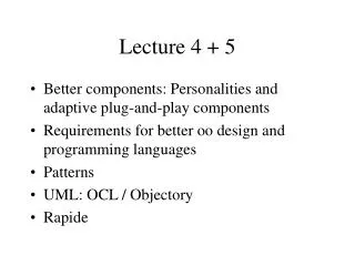
C 110 90 B Output, q, Units per day 56 A 4 6 11 L, Workers per day a MP L 20 , AP b 15 Average product, APL Marginal product, MPL c 11 4 6 L, Workers per day
Between zero and b, MP curve lies above AP curve, causing AP curve to increase. Below b, MP curve is below AP curve, causing AP curve to decrease. Therefore, MP curve must intersect AP curve at maximum point of AP curve. TP increases rapidly up to level of labor input A then increases at a slower rate as labor input increases. TP curve becomes flatter and flatter until it reaches maximum output level at C. Curve implies that marginal product of labor first increases rapidly then decreases, eventually becoming zero or less.
Increasing marginal returns: region where MP curve is positive and increasing Law of diminishing returns: region where marginal product curve is positive but decreasing Negative marginal returns: region where product curve is negative so that TP is decreasing Law of Diminishing Returns : • Occurs because capital input and technologies are held constant • Additional output generated by additional units of variable input (MP) • Production becomes less constrained
Elasticity of production The Relationship between Marginal andAverage Product = + + 11
2. Long-run decisions In the long run, all inputs are variable. Relationship between a flow of inputs and the resulting flow of output where all inputs are variable: Q = f (L, K) where Q = quantity of output L = quantity of labor input (variable) K = quantity of capital input (variable) both inputs are variable
Technical versus Economic Efficiency Technical efficiencyObtaining the greatest possible production of goods and services from available resources. In other words, resources are not wasted in the production process. Technical efficiency is not enough for firms to maximize profits. The firm must choose among the technically efficient options to produce a given level of output at the lowest costEconomic efficiency
Profit Maximization and Cost Minimization For any level of output, maximizing profits requires firms to choose their inputs to minimize total costs. A firm is not minimizing costs if it is possible to substitute one factor for another to keep output constant while reducing total cost: The firm should substitute one factor for another factor as long as the marginal product of one factor per dollar spent on it is greater than the marginal product of the other factor per dollar spent on it.
Labor-intensive method: process that uses large amounts of labor relative to other inputs • Capital-intensive method: process that uses large amounts of capital equipment relative to other inputs • Input substitution: degree to which one input can be substituted for another • Can occur in small-scale or large-scale business • Some processes may not be conducive to substitution • Issue is whether the same quality output is being produced with input substitution • Factors influencing input substitution • Technology • Prices of inputs • Incentives facing a given producer
Isoquant A graph that shows all the combinations of capital and labor that can be used to produce a given amount of output. K 5 3 Q=75 1 2 L
Properties of Isoquants • The farther an isoquant is from the origin, the greater the level of output. • Isoquants do not cross. • Isoquants slope downward Marginal rate of technical substitution (MRTS) The slope of an isoquant, or the rate at which a firm is able to substitute one input for another while keeping the level of output constant.
D K = –6 D L = 1 q = 10 Substitution Among Inputs K a 16 b 10 –3 c 1 7 d –2 1 5 e –1 4 1 0 1 2 3 4 5 6 7 8 9 10 L
Substitutability of Inputs Isoquants When Inputs Are Perfect Substitutes Fixed-Proportions Production Function
Holding the amount of capital fixed at a particular level (say 3), we can see that each additional unit of labor generates less and less additional output.
Isocost line A graph that shows all the combinations of capital and labor available for a given total cost. Slope of isocost line Movements of the isocost line • Change in the budget constraint • The price ratio of the two inputs changes
K Q TC L Finding The Least-cost Technology with Isoquants and Isocosts The firm will choose the combination of inputs that is least costly. The least costly way to produce any given level of output is indicated by the point of tangency between an isocost line (TC) and the isoquant (Q) corresponding to that level of output.
Finding The Least-cost Technology with Isoquants and Isocosts At the point where a line is just tangent to a curve, the two have the same slope. At each point of tangency, the following must be true: Thus, Dividing both sides by PL and multiplying both sides by MPK, we get
MPK 40 MPL 20 = = 4 < = = 10 10 pL 2 pK Example Suppose the marginal product of capital is 40 units of output and the price of one unit of capital is $10. The marginal product of labor is 20 units of output and the price of one unit of labor is $2. In this case, the firm can reduce the cost of producing its current level of output by using more labor and less capital.
How does output respond to increases in all inputs together? Increasing returns to scale – output increases more than in proportion to inputs as the scale of a firm’s production increases. Constant returns to scale – output increases in proportion to inputs as the scale of a firm’s production increases. Decreasing returns to scale – output increases less than in proportion to inputs as the scale of a firm’s production increases.
3. The Very Long Run: Changes In Technology In the very long run, there are changes in the available techniques and resources for firms. Such changes shifts the long-run cost curves. Technological change refers to all changes in the available techniques of production. Economists use the notion of productivity to measure the extent of technological change. Faced with increases in the price of an input, firms may either substitute away (LR) or innovate away (VLR) from the input. These two options can involve different actions and can have different implications for productivity.
Microeconomics Lecture 6 Institute of Economic Theories - University of Miskolc Mónika Kis-Orloczki Assistant lecturer orloczki.monika@uni-miskolc.hu
Explicit costs: payment to an individual that is recorded in an accounting system. Implicit costs: value of using a resource that is not explicitly paid out, is often difficult to measure, and partly not recorded in an accounting system. Economic depreciation measured as the change in the market value of capital over a given period. Normal profitis the return to entrepreneurship. A rate of return on capital that is just sufficient to keep owners and investors satisfied. For relatively risk-free firms, it should be nearly the same as the interest rate on risk-free government bonds.It is part of a firm’s economic cost because it is the cost of the entrepreneur not running another firm. It is the minimum level of profit required to keep the factors of production in their current use in the long run.
Total revenue The amount received from the sale of the product (Q x P). Total cost (total economic cost) The total of explicit (out-of-pocket)andimplicit costs. Accounting profit: difference between total revenue and accountable costs (explicit costs+accountable implicit costs (for exampledepreciation). Economic profit: difference between total revenue and totalcost, both implicit and explicit. = TR - TC
Total revenue Economic profit Total economic costs Explicit cost Implicit costs Normal profit Accountable implicit costs Accounting profit Accountingcosts Costs and revenues of the firm
Short-Run Costsand Output Decisions Fixed cost (FC) Any cost that does not depend on the firm’s level of output. These costs are incurred even if the firm is producingnothing. There are no fixed costs in the long run. Variable cost (VC)A cost that depends on the level of production chosen. Total cost (TC)Fixed costs plus variable costs.
Average fixed cost (AFC)Total fixed cost divided by the number of units of output; aper-unit measure of fixed costs. Average variable cost (AVC) Total variable cost divided by the number of units of output. Average total cost (AC)Total cost divided by the number of units of output.
Marginal cost (MC)The increase in total cost that results from producing one more unit of output. Marginal costs reflect changes in variable costs.
Because fixed costs do not vary with output, the only part of TC that changes is the variable cost. The marginal cost (MC), average total cost (AC), and average variable cost (AVC) curves are all U shaped, and the marginal cost curve intersects the average variable cost and average total cost curves at their minimum points.
MC A AP, MP $ B b AVC AP a MP L Q L1 Q1 L2 Q2 Relation of MP - MC and AP - AVC
Long-run costs Since all inputs are variable, all costs are variable in the long run. Long-run average cost (LRAC) measures the long-run cost of producing one unit of output:
The Relationship between Short-Run Average Cost and Long-Run Average Cost LRAC shows minimum average cost of producing any level of output when all inputs are variable
Return to scale what happens to LRAC as a firm increases its plant size