Divide and Conquer Technique

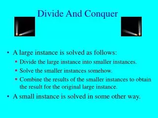
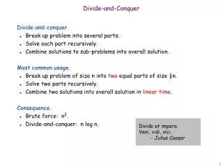
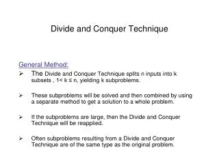
1. Divide and Conquer Technique General Method: The Divide and Conquer Technique splits n inputs into k subsets , 1< k ≤ n, yielding k subproblems. These subproblems will be solved and then combined by using a separate method to get a solution to a whole problem. If the subproblems are large, then the Divide and Conquer Technique will be reapplied. Often subproblems resulting from a Divide and Conquer Technique are of the same type as the original problem.

2. For those cases the reapplication of the Divide and Conquer Technique is naturally expressed by a recursive algorithm. Now smaller and smaller problems of the same kind are generated until subproblems that are small enough to be solved without splitting are produced.

3. Control Abstraction/general method for Divide and Conquer Technique Algorithm DAndC(p) { if Small(p) then return s(p); else { divide p into smaller instances p1,p2,…….,pk, k≥1; Apply DAndC to each of these subproblems; return Combine(DAndC(p1), DAndC(p2),……,DAndC(pk)); } }

4. If the size of problem is n and the sizes of the k subproblems are n1,n2,….,nk,then the computing time of DAndC is described by the recurrence relation T(n)= g( n) n small T(n1)+T(n2)+……+T(nk)+f(n) Otherwise Where T(n) is the time for DAndC on any input of size n and g(n) is the time to compute the answer directly for small inputs. The function f(n) is the time for dividing the problem and combining the solutions to subproblems.

5. The Complexity of many divide-and-conquer algorithms is given by recurrences of the form c n small aT(n/b)+f(n) Otherwise Where a , b and c are known constants. and n is a power of b (i.e n=bk ) T(n)=

6. Applications1.Binary search Algorithm Iterative algorithm Algorithm BinSearch(a,n,x) { low:=1; high:=n; while(low≤high) { mid:=(low+high)/2; if( x<a[mid] ) then high:=mid-1; else if( x> a[mid] ) then low:=mid+1; else return mid; } return 0; }

7. Recursive Algorithm ( Divide and Conquer Technique) Algorithm BinSrch (a,i,l,x) //given an array a [i:l]of elements in nondecreasing //order,1≤i≤l,determine whether x is present,and //if so, return j such that x=a[j]; else return 0. { if(l=i) then // If small(P) { if(x=a[i]) then return i; else return 0; } else { //Reduce p into a smaller subproblem. mid:= (i+l)/2 if(x=a[mid]) then return mid; else if (x<a[mid]) then return BinSrch (a,i,mid-1,x); else return BinSrch(a,mid+1,l,x); } }

8. Time complexity of Binary Seaych If the time for diving the list is a constant, then the computing time for binary search is described by the recurrence relation T(n) = c1 n=1, c1 is a constant T(n/2) + c2 n>1, c2 is a constant Assume n=2k, then • T(n) =T(n/2) + c2 • =T(n/4)+c2+c2 • =T(n/8) +c2+c2+c2 • ….. • ….. • = T(1)+ kc2 • = c1+kc2 =c1+ logn*c2 = O(logn)

9. Time Complexity of Binary Search Successful searches: bestaverage worst O(1) O(log n) O( log n) Unsuccessful searches : bestaverage worst O(log n) O(log n) O( log n)

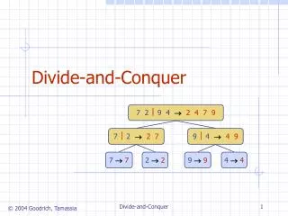
10. 2. Merge Sort • Base Case, solve the problem directly if it is small enough(only one element). • Divide the problem into two or more similar and smaller subproblems. • Recursively solve the subproblems. • Combine solutions to the subproblems.

11. Merge Merge Sort: Idea Divide into two halves A FirstPart SecondPart Recursively sort Recursively sort SecondPart FirstPart A is sorted!

12. Merge-Sort(A, 0, 7) Divide A: 3 7 5 1 6 2 8 4 6 2 8 4 3 7 5 1

13. Merge-Sort(A, 0, 7) , divide Merge-Sort(A, 0, 3) A: 3 7 5 1 8 4 6 2 6 2 8 4

14. Merge-Sort(A, 0, 7) , divide Merge-Sort(A, 0, 1) A: 3 7 5 1 8 4 2 6 6 2

15. Merge-Sort(A, 0, 7) , base case Merge-Sort(A, 0, 0) A: 3 7 5 1 8 4 2 6

16. Merge-Sort(A, 0, 7) Merge-Sort(A, 0, 0), return A: 3 7 5 1 8 4 2 6

17. Merge-Sort(A, 0, 7) , base case Merge-Sort(A, 1, 1) A: 3 7 5 1 8 4 6 2

18. Merge-Sort(A, 0, 7) Merge-Sort(A, 1, 1), return A: 3 7 5 1 8 4 2 6

19. Merge-Sort(A, 0, 7) Merge(A, 0, 0, 1) A: 3 7 5 1 8 4 2 6

20. Merge-Sort(A, 0, 7) Merge-Sort(A, 0, 1), return A: 3 7 5 1 8 4 2 6

21. Merge-Sort(A, 0, 7) , divide Merge-Sort(A, 2, 3) A: 3 7 5 1 2 6 4 8 8 4

22. Merge-Sort(A, 0, 7) Merge-Sort(A, 2, 2), base case A: 3 7 5 1 2 6 4 8

23. Merge-Sort(A, 0, 7) Merge-Sort(A, 2, 2),return A: 3 7 5 1 2 6 4 8

24. Merge-Sort(A, 0, 7) Merge-Sort(A, 3, 3), base case A: 2 6 8 4

25. Merge-Sort(A, 0, 7) Merge-Sort(A, 3, 3), return A: 3 7 5 1 2 6 4 8

26. Merge-Sort(A, 0, 7) Merge(A, 2, 2, 3) A: 3 7 5 1 2 6 4 8

27. Merge-Sort(A, 0, 7) Merge-Sort(A, 2, 3), return A: 3 7 5 1 4 8 2 6

28. Merge-Sort(A, 0, 7) Merge(A, 0, 1, 3) A: 3 7 5 1 2 4 6 8

29. Merge-Sort(A, 0, 7) Merge-Sort(A, 0, 3), return A: 2 4 6 8 3 7 5 1

30. Merge-Sort(A, 0, 7) Merge-Sort(A, 4, 7) A: 2 4 6 8 3 7 5 1

31. Merge-Sort(A, 0, 7) Merge (A, 4, 5, 7) A: 2 4 6 8 1 3 5 7

32. Merge-Sort(A, 0, 7) Merge-Sort(A, 4, 7), return A: 2 4 6 8 1 3 5 7

33. Merge-Sort(A, 0, 7) Merge-Sort(A, 0, 7), done! Merge(A, 0, 3, 7) A: 1 2 3 4 5 6 7 8

34. Ex:- [ 179, 254, 285, 310, 351, 423, 450, 520, 652,861 ] Tree of calls of merge sort 1,10 6,10 1,5 1,3 4,5 6,8 9,10 5,5 10,10 1,2 9,9 4,4 6,7 8,8 3,3 2,2 1,1 7,7 6,6

35. Merge Sort: Algorithm • MergeSort( low,high) • // sorts the elements a[low],…,a[high] which reside in the global array • //a[1:n] into ascending order. • // Small(p) is true if there is only one element to sort. In this case the list is • // already sorted. • {if ( low<high ) then // if there are more than one element • { • mid ←(low+high)/2; • MergeSort(low,mid); • MergeSort(mid+1, high); • Merge(low, mid, high); • } • } Recursive Calls

36. 5 5 15 15 28 28 30 30 6 6 10 10 14 14 5 5 2 3 7 8 1 4 5 6 R: L: 3 5 15 28 6 10 14 22 Merge-Sort: Merge Example high low mid A: B:

37. 5 15 28 30 6 10 14 5 Merge-Sort: Merge Example A: B: 3 1 5 15 28 30 6 10 14 k=low R: L: 3 2 3 15 7 28 30 8 6 1 4 10 5 14 6 22 i=low j=mid+1

38. 5 15 28 30 6 10 14 5 Merge-Sort: Merge Example A: B: 2 1 5 15 28 30 6 10 14 k R: L: 2 3 3 5 7 15 28 8 6 1 10 4 5 14 22 6 i j

39. 5 15 28 30 6 10 14 5 Merge-Sort: Merge Example A: B: 3 1 2 15 28 30 6 10 14 k R: L: 2 3 7 8 1 6 10 4 5 14 6 22 i j

40. 5 15 28 30 6 10 14 5 Merge-Sort: Merge Example A: B: 1 2 3 6 10 14 4 k R: L: 2 3 7 8 1 6 4 10 5 14 22 6 j i

41. 5 15 28 30 6 10 14 5 Merge-Sort: Merge Example A: B: 1 2 3 4 6 10 14 5 k R: L: 2 3 7 8 1 6 10 4 5 14 6 22 i j

42. 5 15 28 30 6 10 14 5 Merge-Sort: Merge Example A: B: 6 1 2 3 4 5 6 10 14 k R: L: 2 3 7 8 1 6 4 10 5 14 6 22 i j

43. 5 15 28 30 6 10 14 5 Merge-Sort: Merge Example A: B: 7 1 2 3 4 5 6 14 k R: L: 2 3 7 8 1 6 4 10 14 5 6 22 i j

44. 5 15 28 30 6 10 14 5 Merge-Sort: Merge Example A: B: 8 1 2 3 4 5 6 7 14 k R: L: 2 3 5 3 7 15 8 28 1 6 4 10 5 14 22 6 i j

45. 5 15 28 30 6 10 14 5 Merge-Sort: Merge Example A: B: 1 2 3 4 5 6 7 8 k R: L: 3 2 3 5 7 15 28 8 6 1 10 4 5 14 6 22 j i

46. 5 15 28 30 6 10 14 5 A: B: 1 2 3 4 5 6 7 8

47. Algorithm Merge(low,mid,high) // a[low:high] is a global array containing two sorted subsets in a[low:mid] // and in a[mid+1:high]. The goal is to merge these two sets into a single set // residing in a [low:high]. b[ ] is a temporary global array. { h:=low; i:=low; j:=mid+1; while( h ≤ mid ) and ( j ≤ high ) do { if( a[h] ≤ a[j] ) then { b[i]:=a[h]; h:=h+1; } else { b[i]:=a[j]; j:=j+1; } i:=i+1; }

48. if( h > mid ) then for k:=j to high do { b[i] := a[k]; i:= i+1; } else for k:=h to mid do { b[i] := a[k]; i:= i+1; } for k:= low to high do a[k]:=b[k]; }

49. Merge-Sort Analysis n n/2 n/2 n/4 n/4 n/4 n/4 2 2 2

50. Merge-Sort Time Complexity If the time for the merging operation is proportional to n, then the computing time for merge sort is described by the recurrence relation n=1, c1 is a constant c1 T(n) = n>1, c2 is a constant 2T(n/2) + c2n Assume n=2k, then • T(n) =2T(n/2) + c2n • =2(2T(n/4)+c2n/2)+cn • =4T(n/4)+2c2n • ….. • ….. • =2k T(1)+ kc2n • = c1n+c2nlogn= = O(nlogn)