Download
1 / 1
10 likes | 179 Views
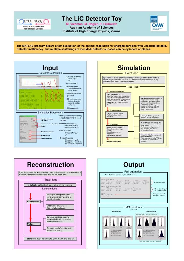
20 Inner Tracker (IT) 21 22 Number of layers : 5 23 Radii [mm] : 90, 90, 160, 300, 340 24 Upper limit in z [mm] : 110, -90, 360, 640, 2730 25 Lower limit in z [mm] : 90,-110, -360, -640,-2730 26 Efficiency Rphi : 0, 0, 0.95, 0.95, 0

E N D
20 Inner Tracker (IT) 21 22 Number of layers : 5 23 Radii [mm] : 90, 90, 160, 300, 340 24 Upper limit in z [mm] : 110, -90, 360, 640, 2730 25 Lower limit in z [mm] : 90,-110, -360, -640,-2730 26 Efficiency Rphi : 0, 0, 0.95, 0.95, 0 27 Efficiency 2nd layer (eg. z) : -1, -1, 0.95, 0.95, -1 28 Stereo angle alpha [Rad] : 10*pi/180 29 Thickness [rad. lengths] : 0.07,0.07,0.0175,0.0175, 0.14 30 error distribution : 1 31 0 normal-sigma(RPhi) [1e-6m] : 32 sigma(z) [1e-6m] : 33 1 uniform-d(RPhi) [1e-6m] : 50 34 d(z) [1e-6m] : 50 Number of events rsp. tracks Momentum and direction Vertex Simulation features Test features Output features The MATLAB program allows a fast evaluation of the optimal resolution for charged particles with uncorrupted data. Detector inefficiency and multiple scattering are included. Detector surfaces can be cylinders or planes. The LiC Detector ToyM. Valentan, M. Regler, R. FrühwirthAustrian Academy of SciencesInstitute of High Energy Physics, Vienna Input Simulation Detector Description Event loop • Coaxial cylinders - Stereo angle - in T • PC z dependent • Plane wheels - Coordinates defined by two angles • Arbitrary size and position • 2D measurement - single and passive layers steered by inefficiency • Strips or pads By default the event loop first generates a vertex (uniformly distributed in a certain range). However, the user can enter the vertex positions (x0,y0,z0), provided by an arbitrary vertex generator. Trackloop Frame Detector 1 Detector 2 Momentum variables Track parameters,, (according to the chosen multiplicity). The state vector is propagated to the beam tube, where it is transformed to variables similar to the DELPHI-convention,z,, including spatial variables. Multiple scattering takes place on every massive barrier, using independent normal distributed random quantities (according to the Highland formula). A local cartesian coordinate system is used with one axis tangent to the track. Track simulation Simulation Parameters The track model is a helix. Tracking includes multiple scattering. Arbitrary inefficiency without spatial or angular dependence • Start parameters uniformly distributed in the defined ranges • Simulation features: - Multiple scattering - Measurement errors • Test features:- Pulls and MC-pulls - ² • Output features: - Histograms of pulls - Histograms of residuals - 6D cartesian, Harvester Strip detectors (single layer and double sided; inner layer with any stereo angle) Pixel detectors (by crossing 2 strip detectors with strictly correlated inefficiency) Coordinates Measurement of R and z' (according to stereo angle chosen) Strips, Pads or normal distributed uncorrupted data only Simulation of digital and normal distributed errors. The z dependence in the TPC can be used as an example for a template. Reconstruction Reconstruction Output Pull quantities Track fitting uses the Kalman filter, a recursive least-squares estimator. It proceeds from the outermost layer towards the beam tube. Test statistics (sample log file, 10000 tracks) Monte-Carlo pulls Phi z theta beta kappa mean: -0.0014137 -0.020775 0.006437 -0.0035657 -0.0024358 std: 0.99745 1.0021 0.99926 0.99836 0.997 Pulls at innermost detector RPhi z u v mean: 0.0085271 0.0029371 -0.0095907 0.0042998 std: 0.99706 0.998 1.0031 1.0088 Chi^2 ndf: 21.8725 mean: 21.9226 Track loop At the beam tube Initialization of the track parameters with large errors Detector loop R, z – barrel region u,v - forward region Average number of degrees of freedom Propagate track parameters, using a reference track and a linearized model Extrapolation Linear error propagation Add multiple scattering MC residuals (fitted - true) Barrel region Forward region Scale factor relative to the barrel region: 50 Compute weighted mean of extrapolated track parameters and measurement Update Compute local χ2 statistic and accumulate total χ2 10000 track with 0.7454<2.3562 Up: Monte-Carlo residuals at the beam tube, computed from generated and fitted state vectors Left: Relative deviation pT/pT Right: Relative deviation pT/pT2 10000 track with 0.49087<0.098175 Up: Monte-Carlo residuals at the beam tube, computed from generated and fitted state vectors Left: Relative deviation pT/pT Right: Relative deviation pT/pT2 Store final track parameters, error matrix and total χ2 Scale factor relative to the barrel region: 100