Download
1 / 23
240 likes | 417 Views
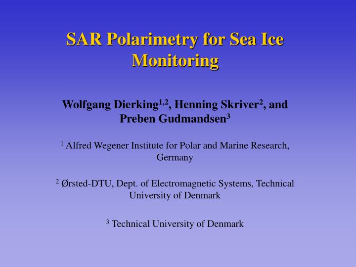
SAR Polarimetry for Sea Ice Monitoring. Wolfgang Dierking 1,2 , Henning Skriver 2 , and Preben Gudmandsen 3 1 Alfred Wegener Institute for Polar and Marine Research, Germany 2 Ørsted-DTU, Dept. of Electromagnetic Systems, Technical University of Denmark 3 Technical University of Denmark.

E N D
SAR Polarimetry for Sea Ice Monitoring Wolfgang Dierking1,2, Henning Skriver2, and Preben Gudmandsen3 1 Alfred Wegener Institute for Polar and Marine Research, Germany 2Ørsted-DTU, Dept. of Electromagnetic Systems, Technical University of Denmark 3 Technical University of Denmark
ESA POLSAR ProjectSea Ice Study Our presentation focusses on two questions: • Do we gain anything by utilising polarimetric data (intensities + phase differences) in sea ice classification ? • What is the optimal strategy for sea ice classification ?
Data Sets We utilised airborne SAR imagery from the flight campaigns listed below: • AIRSAR: Beaufort Sea (March 1988), L+C-band • EMISAR: Greenland Sea (March 1995), C-band • EMISAR: Baltic Sea (March 1995), L+C-band (EMAC campaign) (Winter conditions, ice regimes at the 3 sites are different from one another.)
Polarimetric Phase HHVV • Including HHVV and HHVV in a sea ice classification scheme does not significantly improve the classification accuracy. (Rignot and Drinkwater, 1994) • Thin ice areas often reveal a HHVV significantly different from zero. Is HHVV linked to the thickness of thin ice ? (Winebrenner et al., 1995; Thomsen et al., 1998a,b; Thomsen, 2001) • A fully polarimetric model (intensity and phase) has been used to retrieve thin ice thickness by means óf a neural network. Result: C-band data seems to work for thicknesses 0-10cm, L-band is less sensitive. Contribution of individual polarization coefficients ? (Kwok et al., 1995)
Intensity R-0XP, G-0HH, B-0VV Co-polarisation Ratio 0VV / 0HH Phase HHVV Versus Intensity Example 1 Greenland Sea C-Band Depolarisation Ratio 0HV / (0HH + 0VV) Phase Difference HHVV
Intensity R-0XP, G-0HH, B-0VV Co-polarisation Ratio 0VV / 0HH Phase Difference HHVV Phase HHVV Versus Intensity- Example 2 Greenland Sea, C-Band
Phase difference HHVV Observations 1
Thin Ice Radar Signatures C-band scatterometer measurements over growing ice in a cold room at CRREL: Backscattered intensity at like- and cross- polarisation increased by 6-10 dB as the ice thickened from 3cm to 11cm. (Nghiem et al., 1997) TH1 TH2 TH3 TH4
Phase Difference HHVV • Improves classification: discrimination thin ice – open water • Linked with thin ice thickness ? (classification, heat and salt fluxes) • Needs further research: what determines the magnitude of HHVV ? (brine inclusions, anisotropic volume – scattering from the ice-water interface, dielectric profile)
Sea Ice Classification Our choice is a hierarchical scheme (knowledge-based approach) WHY ? • Results of measurements and theoretical modelling of sea ice radar signatures, and the experience gained from field campaigns can be considered. • Decision boundaries at the individual levels in the hierarchy can be determined by means of statistical methods. (A similar procedure is applied at the ASF, Kwok et al., 1991)
Methodology: Step 1 • We determined „typical“ values of various polarimetric parameters for different ice types visually (subjectively) identified in the radar images. • Polarimetric parameters: • Covariance matrix: intensities VV, HH, XP, correlation and phase • difference HHVV, co- and depolarisation ratio, symmetry. • Decomposition (coherency matrix): entropy, alpha, anisotropy. Visual classification on the basis of • a 3-layer image format representing only intensities (R-HV, G-HH, B-VV) • complementary data (photos, videos, in-situ spot measurements, meteorological data).
Greenland Sea Baltic Sea Polarimetric parameters of different ice types - Example Beaufort Sea
Methodology: Step 2 For the classification scheme, polarimetric parameters have been selected for which distance between ice type data clusters is largest
Methodology: Step 3 We devised classification rules for each test site and radar band Classification Rules for Greenland Sea Ice (Winter)
Classification, Greenland Sea, C-Band Hierarchical Approach, ISODATA thresholds Intensity R(HV) G(HH) B(VV)
Classification, Greenland Sea, C-Band Used Parameters: 0HV, HHVV 0VV / 0HH 0HV / (0VV + 0HH) Classes: 1 Ridged ice (39) 2 MY ice 1(141) 3 MY ice 2 (98) 4 Thin ice 1-3 (101) 5 Thin ice 4 (49) 6 Open Water (33) Confusion matrix for hierarchical classification: 1 2 3 4 5 6 1 100.0 0.0 0.0 0.0 0.0 0.0 2 0.0 98.5 0.7 0.7 0.0 0.0 3 0.0 7.9 92.1 0.0 0.0 0.0 4 0.0 0.9 13.4 84.8 0.9 0.0 5 0.0 0.0 0.0 9.4 90.6 0.0 6 0.0 0.0 0.0 0.0 0.0 100.0 Confusion matrix for ISODATA with hierarchical classification as initialisation: 1 2 3 4 5 6 1 100.0 0.0 0.0 0.0 0.0 0.0 2 0.0 99.3 0.0 0.7 0.0 0.0 3 0.0 4.5 93.3 2.2 0.0 0.0 4 0.0 0.9 11.6 86.6 0.9 0.0 5 0.0 0.0 1.9 5.7 92.5 0.0 6 0.0 0.0 0.0 0.0 0.0 100.0
Classification: Decomposition • Indicates scattering • mechanisms from sea ice: • Z9, Z6: surface scattering • with an increasing amount • of secondary scattering • contributions • Z8, Z5: volume scattering • from inclusions with a • decreasing correlation of • their orientation • Z2: noise-like scattering • from randomly oriented • scatterers
Sea Ice Classification • Regional and seasonal differences in ice cover characteristics require different „optimal“ sequences of classification rules (are they stable for a particular region and season ?).
Which frequency, which polarisations ? X-band (intensity) is very similar to C-band