Q2D Turbulence by Rayleigh-Taylor Instabilities

1. Q2D Turbulence by Rayleigh-Taylor Instabilities Xi Li and Vincent H. Chu Dept. of Civil Engineeringand Applied Mechanics McGill University 4th International Symposium on Environmental Hydraulics December 15,2004

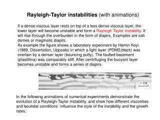
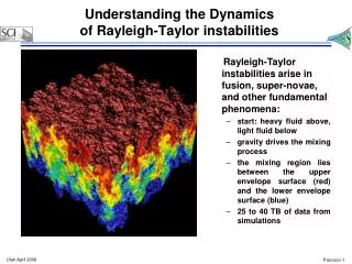
2. Objectives and Method • Experimental study of the Rayleigh-Taylor instabilities by sudden overturning a tank of stably stratified fluid of two layer • Interfacial mixing is determined accurately by measuring the tracer dye concentration using a video imaging technique • Provide the data for the development of LES (Large Eddy Simulation) model

3. h1 h2 1800 T L Overturning a Tank of Two-Layer Fluid

4. Late Stage Development when d >> h1 d = a(2gAh1)1/2 t (1) where g = gravity constant, h1 = initial depth of the upper layer, A = (r1 - r 2)/( r 1 + r 2) = Atwood number, and 2gAh1 = total buoyant force associated with the upper layer

5. General Development: s = fn (t, g’, h1) Length scale = h1Time scale ts= (h1 /g’)1/2 where g’ = reduced gravity, h1 = initial depth of the upper layer, s = layer thickness

6. Quadratic in the Initial Stage and Linear in the Late Stage of Development Length scale = h1Time scale ts= (h1 /g’)1/2

7. Mixing Thickness by Gaussian Profile (2) whereC= mean tracer dye concentration determined by the video imaging method, Cm = maximum of the mean, d = mixing layer thickness defined by concentration profile

8. Tracer Dye Concentration at t = 9 s

9. Data at t = 9 s by the Gaussian profile

10. Tracer dye concentration at t = 13 s

11. Date at t = 13 s by the Gaussian profile

12. Mixing layer thickness d versus time t.

13. Fittingdata with d = a(2gAh1)1/2 t a = 0.13

14. The coefficient a __________________________________________________________________________________________________________________________________________________________________ Time (s) depth d (cm) coefficient a ________________________________________________________________________ 9 6.1700 0.13 10 7.1947 0.14 11 7.6056 0.13 12 8.5235 0.13 13 9.2586 0.13 14 10.2756 0.14 15 11.2919 0.13 _________________________________________________________________________ The coefficient a = 013 based on the tracer dye concentration measurements is significantly smaller than the value of 0.38 obtained based on the visual inspection by Voropayev et al. (1993).

15. Large Eddy Simulation (LES) Simulation uses the four-third-power interpolation formula in the modified Smagorinsky model proposed by Babarutsi, Nassiri and Chu (2004):

16. If then If then Modified Smagorinsky Viscosity

17. Largrangian Block Method (LBM) The LBM is a highly accurate numerical scheme that is relatively free of numerical diffusion and unphysical oscillations. Similarly successful simulations of highly turbulence interfaces have been obtained by the method using the method for a variety of the turbulent flows (see, e.g., Chu and Altai 2002).

18. Large Eddy Simulation at t = 9 s

19. LES with Experimental data at t = 9 s

20. Large Eddy Simulation at t = 15 s

21. LES with Experimental data at t = 15 s

22. Conclusion • Successful simulation of a highly irregular turbulent interface due the Rayleigh-Taylor instability has been obtained using the Lagrangian Block Method. • The results are highly consistent with the laboratory data obtained from an overturn experiment. • The LBM is positive definite and relatively free of the numerical oscillation and diffusion. It is shown in the present investigation to be suitable for simulation of highly complex turbulence interfaces.