Download
1 / 34
340 likes | 564 Views
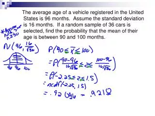
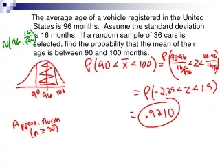
SAMPLING DISTRIBUTION MODELS for Proportions Ch. 7. A study found that young women in America had an average height of 64.5 inches with a standard deviation of 2.5 inches.

E N D
A study found that young women in America had an average height of 64.5 inches with a standard deviation of 2.5 inches. If 10 young women (assume that they are independent of one another) were to come into the classroom, what kind of heights would you expect to see? What average height would you expect to see for those 10 women? Will the distribution for the 10 women be normally distributed? Perform a simulation to see… Young Women’s Heights
Materials: Several 3” x 3” Post-it Notes, TI-83 plus Use the operation randNorm(64.5, 2.5, 10) in the header of the six lists. Find the mean, median, and standard deviation of each list. Graph the distributions – describe it (remember a good description of a distribution is Shape, Center, Spread, and Outliers!) (An example of the model) Young Women’s Heights
Sampling Distributions – What’s the point? On October 27, 2000, less than two weeks before the presidential election, an NBC poll reported that from 1000 randomly selected registered voters, that 45% showed support for Gore and 43% favored Bush. A CNN poll stated that 46% supported Bush and 42% supported Gore. Why are the numbers off? Does this mean that CNN has better polling techniques than NBC (since Bush won)? We know that there is always variance, but how much should we expect to see? Sampling Distributions help to answer these questions. Sample Distributions
A random sample of 160 High School students at a certain school were asked whether they had taken any form of drugs including alcohol and tobacco. Of the respondents, 105 said “Yes.” So the proportion of the sample who said they had taken some form of drug was If another sample was taken, would it yield the exact same results? Why or why not? Can you say that the proportion of the students that take drugs at this school is absolutely 65.6%? Obviously not, this notion is the key concept to this lesson! Example: Have you taken drugs?
Sample Distributions • If you continued to take a sample of 160 students from this particular high school, each sample would have a slightly different proportion (although the values would be close to one another, they won’t all be exactly the same).This is an example of sampling variability: the value of a statistic varies in repeated random sampling. This variability is the reason that we consider a sample statistic to be a random variable whose distribution merits investigation. • Assume that the true proportion of students that had taken some form of drug was 64%. Is 65.6% far from what we should expect? • Although our estimate is a little too high, 65.5% as opposed to 64%, it is consistent with what we should expect from just one random sample. We will examine how likely or unlikely these types of events are in this chapter. • This is what is sometimes called Sampling Error. It’s not really an error, but usual variability that you would expect to see from one sample to the next. Sampling Variabilitymight be a better word.
The sampling distribution model of a statistic is the distribution of values taken by the statistic in all possible samples of the same size from the same population. Using the Law of Large Numbers, Pierre-Simon Laplace was able to examine the Sampling Distribution model and come up with the Central Limit Theorem, or the CLT…an amazing discovery that shocked the mathematical world in the late 1700’s… Sample Distributions
The Central Limit Theorem (CLT) • According to the CLT, sampling distribution MODELS for ANY mean or proportions become Normal as n increases. • This Theorem is also called the Fundamental Theorem of Statistics (because…YES, it’s that important!!!) • The CLT does not talk about the distribution of data within a sample. It talks about all the different samples drawn from the same population, or the sampling distribution model.
Be careful not to think that the CLT says that the sample data will be normal, far from it! The sample data will look more and more like the population from which it is drawn as the sample get larger. The CLT guarantees that each sampling distribution is going to be Normal as long as the sample is large enough!!! The strangest and most controversial aspect of the CLT is that the sampling distribution model becomes more Normal as the sample size increases regardless of the shape of the population distribution (skewed, bimodal, or any other distribution) – this caused quite a stir in many mathematics circles when it was first introduced. The Central Limit Theorem (CLT)
The Central Limit Theorem (CLT) • There are two assumptions that must be satisfied in order for the CLT to work: • Independence Assumption: The sampled values must be mutually independent. Once again, there is no way to check this for sure, so we check this assumption by satisfying the two conditions: randomization condition – we check to see if the values of the sample were taken from a random selection of the population and 10% condition– the sample size is no more than 10% of the population. • Large Enough Sample Assumption: The larger the sample, the more normal the distribution. We need to make sure that
The Normality of Sampling Distribution • A little more about Assumptions… • Assumptions are almost impossible to verify (that’s why we assumethat they are true). However, we want to make sure that our assumptions are justified, so we always check the conditions that allow us to safely make the assumption. • For the independence assumption, check randomization and the 10% condition • If the sample is not a random selection, then independence can easily be violated. One of the best strategies of ensuring independence is randomization. • Once you take more than 10% of the population, the probabilities show a marked difference causing us to violate our independence assumption. Although we may violate the independence assumption in various ways, it is important to always check this condition.
The Normality of Sampling Distribution • A little more about Assumptions… • Assumptions are almost impossible to verify (that’s why we assume that they are true). However, we want to make sure that our assumptions are justified, so we always check the conditions that allow us to safely make the assumption. • For the large enough sample assumption, we check the success/failure condition • We need to make sure that This condition allows us to say that the sample is large enough to have a Normal Sampling Model (by the CLT).
The Normality of Sampling Distribution If you think about the independence and large enough sample assumptions and conditions, they seem somewhat contradictory. On the one hand, we want to make sure that the sample is less than 10% of the population (not too large); and on the other hand, we want to make sure that our sample is large enough to make sure that the np and nq are greater than 10 (a large sample). A good way to think about it is make sure that your sample is big, but not too big. These are two main assumptions and the conditions we check to get information about our sampling distribution. Get use to always checking your conditions from this point on out!!!
The Sampling Distributions of P-Hat • The mean of the sampling model is exactly p: =p • The standard deviation of the sampling distribution model is • Back to Gore and Bush: • Let’s suppose that the true proportion that supported Gore was 42%. NBC used a sample of 1000 randomly selected registered voters: • What is the mean of our sampling distribution? • What is the standard deviation of the sampling distribution?
Back to Gore and Bush: NBC reported that from 1000 randomly selected registered voters, that 45% showed support for Gore. But, this is just one sample. If we conducted another poll, would we obtain the exact same results? Each of our samples will be relatively close to 42% (the true mean), but we should expect variability from one sample to the next. Approximately 95% of all the samples will be within what range? (Use the empirical rule). Since 95% of the samples will be within ±2σ, we should expect to get samples from .42 ± 2(.0156) ≈ .3888 to .4512 about 95% of the time. The Sampling Distribution
The variability of a statistic is described by the spread of its sampling distribution. This spread is determined by the sampling design and the size of the sample. Larger samples give smaller spread. Why do you think this is? The size of the sampleis much more important than the size of the population. A sample of 10 from a group or 100 people is the same as a sample of 10 from a group of 1000! (look at pg. 424) Earlier we stated that as long as the sample is large enough, then the sampling distribution is approximately normal. But, what do we consider large enough? Remember the Success/Failure condition… np ≥ 10 and nq ≥ 10 (any sample with at least 10 success and 10 failures is considered large enough!) If the sample is not large enough, then the model looks like the parent population Variability of a Statistic
Ex 1: Sampling Distributions for Proportions • The Census Bureau reports that 40% of the 50,000 families in a particular region have more than one color TV in their household. What is the probability that a simple random sample (SRS) of size 100 will indicate 45% or more households with more than one color TV when the true population proportion is 40%? • We will follow a FOUR-STEP PROCESS… • First, state what you want to knowand determine what the question is asking (this should always be your first step from this point out): • We want to determine the probability of obtaining an SRS of size 100 that has 45% or more of its households with more than one color TV within a certain population.
Ex 1: Sampling Distributions for Proportions • The Census Bureau reports that 40% of the 50,000 families in a particular region have more than one color TV in their household. What is the probability that a simple random sample (SRS) of size 100 will indicate 45% or more households with more than one color TV when the true population proportion is 40%? • Second, examine the assumptions and check the conditions: • Independence Assumption • Randomization Condition: We are given that the sample was a random selection. • 10% condition: We are told that there are 50,000 families in this particular region. Our sample of 100 is definitely less than 10% of the population.
Ex 1: Sampling Distributions for Proportions • The Census Bureau reports that 40% of the 50,000 families in a particular region have more than one color TV in their household. What is the probability that a simple random sample (SRS) of size 100 will indicate 45% or more households with more than one color TV when the true population proportion is 40%? • Second, examine the assumptions and check the conditions: • Large Enough Sample Assumption • Success/Failure condition:np = (100)(.40)=40 and nq = 100(.60)=60. Both are greater than 10.
Ex 1: Sampling Distributions for Proportions • The Census Bureau reports that 40% of the 50,000 families in a particular region have more than one color TV in their household. What is the probability that a simple random sample (SRS) of size 100 will indicate 45% or more households with more than one color TV when the true population proportion is 40%? • Third, state the parameters and show your work– since we know that we satisfy our conditions, • We will have an approximately normal distribution. • The population mean was given: • The standard deviation can found using the formula: • The model for is N(.40, .049)
Ex 1: Sampling Distributions for Proportions • The Census Bureau reports that 40% of the 50,000 families in a particular region have more than one color TV in their household. What is the probability that a simple random sample (SRS) of size 100 will indicate 45% or more households with more than one color TV when the true population proportion is 40%? • Third, state the parameters and show your work: • Calculate P( ≥ 0.45). • z - score,
Ex 1: Sampling Distributions for Proportions • The Census Bureau reports that 40% of the 50,000 families in a particular region have more than one color TV in their household. What is the probability that a simple random sample (SRS) of size 100 will indicate 45% or more households with more than one color TV when the true population proportion is 40%? • Third, state the parameters and show your work: • Find the probability that z ≥ 1.02. • normalcdf (1.02, E99, 0, 1) or normalcdf (1.02, E99) • Instead of using the z-score, we could just use normalcdf (.45, E99, .4, .049) ≈ 0.15 • Although the z-score step is unnecessary, AP readers love to see the z-score in action. My advice, if you can use the z-score without getting confused or wasting too much time, use it. • normalcdf (1.02, E99) ≈ 0.15
Ex 1: Sampling Distributions for Proportions • The Census Bureau reports that 40% of the 50,000 families in a particular region have more than one color TV in their household. What is the probability that a simple random sample (SRS) of size 100 will indicate 45% or more households with more than one color TV when the true population proportion is 40%? • Fourth, last but not least, state your conclusion in context of the problem: • There is a probability of roughly 0.15 that a sample of size 100 will have a proportion of 0.45 or more when the population proportion is 0.40. A sample proportion of 0.45 is not necessarily an unexpected event and could easily occur simply by sampling variation.
Beware of observations that are not independent! The CLT depends on the assumptions of independence. Unfortunately, this isn’t something you can check in your data. You have to think about how the data were gathered. Good sampling practice and well-designed randomized experiments assure independence. Watch out for small samples from skewed populations! The CLT assures us that the sampling distribution model is approximately Normal if n is large enough. If the population is normal, then we don’t need to worry, but if the population is very skewed, then n will need to be large enough for the distribution to be Normal. Unfortunately, there is no good rule of thumb. It just depends on how skewed the population is. Common Errors
Don’t confuse sampling distribution models with the distribution of a single sample! The sampling distribution model is an imaginary collection of the values that a statistic might have taken from ALL the random samples that you can get. We use the sampling distribution model to make statements about how the statistic varies. Common Errors
Ex: Sampling Distributions for Proportions • Let’s imagine that we conduct a survey and find that 52% of voters plan to vote “Yes” on the upcoming school budget. Our poll is a random sample of 300 voters. What is the percentage of yes-voters for the population? • We will follow a FOUR-STEP PROCESS… • First, state what you want to know and determine what the question is asking (this should always be your first step from this point out): • We want to find the population proportion that may vote “Yes” on the upcoming school budget.
Ex: Sampling Distributions for Proportions • Let’s imagine that we conduct a survey and find that 52% of voters plan to vote “Yes” on the upcoming school budget. Our poll is a random sample of 300 voters. What is the percentage of yes-voters for the population? • Second, examine the assumptions and check the conditions: • Independence Assumption • Randomization Condition: We are given that the sample was a random selection. • 10% condition: Of all the voters in the upcoming election, there are probably more than 3000 people, so it is safe to assume that the samples are independent.
Ex: Sampling Distributions for Proportions • Let’s imagine that we conduct a survey and find that 52% of voters plan to vote “Yes” on the upcoming school budget. Our poll is a random sample of 300 voters. What is the percentage of yes-voters for the population? • Second, examine the assumptions and check the conditions: • Large Enough Sample Assumption • Success/Failure condition: np = (300)(.52)=156 and nq = 300(.48)=144. Both are greater than 10.
Ex: Sampling Distributions for Proportions • Let’s imagine that we conduct a survey and find that 52% of voters plan to vote “Yes” on the upcoming school budget. Our poll is a random sample of 300 voters. What is the percentage of yes-voters for the population? • Third, state the parameters and show your work – since we know that we satisfy our conditions, we will have an approximately normal distribution. • The population mean was given: • The standard deviation can found using the formula: • Provide a graph (this should be done as much as possible) • The model for is N(.52, .029)
Ex: Sampling Distributions for Proportions • Let’s imagine that we conduct a survey and find that 52% of voters plan to vote “Yes” on the upcoming school budget. Our poll is a random sample of 300 voters. What is the percentage of yes-voters for the population? • Fourth, last but not least, state your conclusion in context of the problem: • According to the empirical rule of the Normal model, we expect 68% of the samples of 300 voters to have proportions of “Yes”-voters between 0.491 and 0.549, 95% of the samples to have proportions between 0.462 and 0.578, and 99.7% of the samples to have proportions between 0.433 and 0.607.
Ex: Sampling Distributions for Proportions • Let’s imagine that we conduct a survey and find that 52% of voters plan to vote “Yes” on the upcoming school budget. Our poll is a random sample of 300 voters. What is the percentage of yes-voters for the population? • You will follow this four-step procedure from now on out – get use to it! • I will grade all of your work according to this process from now on out, if you miss a step, you will lose points! These are the steps that every good inference procedure takes!
Means and Standard Deviation As long as the sample is large enough, the sampling distribution model will be approximately normal with mean of μ or p, for means or proportions respectively, and a standard deviation that is dependent on the size of the sample.