Download

1 / 63
630 likes | 639 Views
Chapter 8 The Gain From Portfolio Diversification. Level of Risk. Determine. Optimal Portfolio. Expected Return. Background Assumptions. As an investor you want to maximize the returns for a given level of risk. The relationship between the returns for assets in the portfolio is important.

E N D
Level of Risk Determine Optimal Portfolio Expected Return
Background Assumptions • As an investor you want to maximize the returns for a given level of risk. • The relationship between the returns for assets in the portfolio is important. • A good portfolio is not simply a collection of individually good investments.
Risk Aversion Given a choice between two assets with equal rates of return, risk averse investors will select the asset with the lower level of risk.
Evidence ThatInvestors are Risk Averse • Many investors purchase insurance for: Life, Automobile, Health, and Disability Income. The purchaser trades known costs for unknown risk of loss • Yield on bonds increases with risk classifications from AAA to AA to A….
Are all investors risk averse? Risk preference may have to do with how skewed the possible returns are that are involved - risking small amounts, but insuring large losses Do the possible outcomes push the investor into different categories of overall consumption?
Definition of Risk 1. Uncertainty of future outcomes or 2. Probability of an adverse outcome We will consider several measures of risk that are used in developing portfolio theory
Markowitz Portfolio Theory • Formally extends the MVC from individual stocks to a portfolio context • Quantifies risk • Derives the expected rate of return for a portfolio of assets and an expected risk measure • Shows the variance of the rate of return is a meaningful measure of portfolio risk • Derives the formula for computing the variance of a portfolio, showing how to effectively diversify a portfolio
Assumptions of Markowitz Portfolio Theory 1. Investors consider each investment alternative as being presented by a probability distribution of expected returns over some holding period.
Assumptions of Markowitz Portfolio Theory 2. Investors minimize one-period expected utility, and their utility curves demonstrate diminishing marginal utility of wealth.
Assumptions of Markowitz Portfolio Theory 3. Investors estimate the risk of the portfolio on the basis of the variability of expected returns.
Assumptions of Markowitz Portfolio Theory 4. Investors base decisions solely on expected return and risk, so their utility curves are a function of expected return and the expected variance (or standard deviation) of returns only.
Assumptions of Markowitz Portfolio Theory 5. For a given risk level, investors prefer higher returns to lower returns. Similarly, for a given level of expected returns, investors prefer less risk to more risk. (MVC) Are these assumptions realistic? Do investors really act to “maximize their utility functions w.r.t. expected return and variance”? Do pool players pay attention to the rules and laws of physics?
Assumptions of Markowitz Portfolio Theory Using these five assumptions, a single asset or portfolio of assets is considered to be efficient if no other asset or portfolio of assets offers higher expected return with the same (or lower) risk, or lower risk with the same (or higher) expected return.
Alternative Measures of Risk • Variance or standard deviation of expected return • Alternatively, variation away from some benchmark (tracking error) • Range of returns • Returns below expectations • Semivariance - measure expected returns below some target • Intended to minimize the damage
Expected Rates of Return • Individual risky asset • Sum of probability times possible rate of return • Portfolio • Weighted average of expected rates of return for the individual investments in the portfolio
Computation of Expected Return for an Individual Risky Investment
Computation of the Expected Return for a Portfolio of Risky Assets
Variance (Standard Deviation) of Returns for an Individual Investment Standard deviation is the square root of the variance Variance is a measure of the variation of possible rates of return Ri away from the expected rate of return [E(Ri)]
Variance (Standard Deviation) of Returns for an Individual Investment where Pi is the probability of the possible rate of return, Ri
Variance (Standard Deviation) of Returns for an Individual Investment Standard Deviation
Variance (Standard Deviation) of Returns for an Individual Investment Variance ( 2) = .0050 Standard Deviation ( ) = .02236
Variance (Standard Deviation) of Returns for a Portfolio Computation of Monthly Rates of Return
Variance (Standard Deviation) of Returns for a Portfolio For two assets, i and j, the covariance of rates of return is defined as: Covij = E{[Ri - E(Ri)][Rj - E(Rj)]}
Computation of Covariance of Returns for Coca-Cola and Exxon: 1998
Scatter Plot of Monthly Returns for Coca-Cola and Exxon: 1998
Computation of Standard Deviation of Returns for Coca-Cola and Exxon: 1998
Portfolio Standard Deviation Calculation • Any asset of a portfolio may be described by two characteristics: • The expected rate of return • The expected standard deviations of returns • The correlation, measured by covariance, affects the portfolio standard deviation • Low correlation reduces portfolio risk while not affecting the expected return
Combining Stocks with Different Returns and Risk Case Correlation Coefficient Covariance a +1.00 .0070 b +0.50 .0035 c 0.00 .0000 d -0.50 -.0035 e -1.00 -.0070 1 .10 .50 .0049 .07 2 .20 .50 .0100 .10
Combining Stocks with Different Returns and Risk • Assets may differ in expected rates of return and individual standard deviations • Negative correlation reduces portfolio risk • Combining two assets with -1.0 correlation reduces the portfolio standard deviation to zero only when individual standard deviations are equal
Constant Correlationwith Changing Weights 1 .10 rij = 0.00 2 .20
Portfolio Risk-Return Plots for Different Weights E(R) 2 With two perfectly correlated assets, it is only possible to create a two asset portfolio with risk-return along a line between either single asset Rij = +1.00 1 Standard Deviation of Return
Portfolio Risk-Return Plots for Different Weights E(R) f 2 g With uncorrelated assets it is possible to create a two asset portfolio with lower risk than either single asset h i j Rij = +1.00 k 1 Rij = 0.00 Standard Deviation of Return
Portfolio Risk-Return Plots for Different Weights E(R) f 2 g With correlated assets it is possible to create a two asset portfolio between the first two curves h i j Rij = +1.00 k Rij = +0.50 1 Rij = 0.00 Standard Deviation of Return
Portfolio Risk-Return Plots for Different Weights E(R) With negatively correlated assets it is possible to create a two asset portfolio with much lower risk than either single asset Rij = -0.50 f 2 g h i j Rij = +1.00 k Rij = +0.50 1 Rij = 0.00 Standard Deviation of Return
Portfolio Risk-Return Plots for Different Weights E(R) Rij = -0.50 f Rij = -1.00 2 g h i j Rij = +1.00 k Rij = +0.50 1 Rij = 0.00 With perfectly negatively correlated assets it is possible to create a two asset portfolio with almost no risk Standard Deviation of Return
The Efficient Frontier • The efficient frontier represents that set of portfolios with the maximum rate of return for every given level of risk, or the minimum risk for every level of return • Frontier will be portfolios of investments rather than individual securities • Exception: the asset with the single highest return
Efficient Frontier for Alternative Portfolios Efficient Frontier B E(R) A C Standard Deviation of Return
The Efficient Frontier and Investor Utility • An individual investor’s utility curve specifies the trade-offs he is willing to make between expected return and risk • The slope of the efficient frontier curve decreases steadily as you move upward • These two interactions will determine the particular portfolio selected by an individual investor
The Efficient Frontier and Investor Utility • The optimal portfolio has the highest utility for a given investor • It lies at the point of tangency between the efficient frontier and the utility curve with the highest possible utility
Selecting an Optimal Risky Portfolio Figure 8.10 U3’ U2’ U1’ Y U3 X U2 U1
Gains From Diversification • Lower Correlation • Smaller Portfolio Variance • Larger Gains From Diversification • For a Given Set of Weights
How Many Stocks Are Required For Adequate Diversification? • Benefits achieved even with “naïve” or evenly weighted diversification • The More Stocks, the Better • Increasing Transaction Costs • 10-15 Stocks Sufficient • 90% of Maximum Benefit with 12-18 • Most Benefits Achieved with 10 • Diminishing Benefits with Additional Stocks
“A Little Diversification Goes A Long Way” As the Number of Assets Increases the Incremental Contribution to Variance Reduction Becomes Smaller and Smaller
Mutual Funds • Diminishing Benefits of More Stocks are Still Positive • There is some gain • Low Cost of Data • Large Funds Have to Invest in Many Stocks • Avoid buying and selling affects • Regulation M • Own 5% of any company’s stock