Download
1 / 40
430 likes | 670 Views
Southern Ocean Fronts and eddies. Plan : Monitoring frontal movements in the Southern Ocean with altimetry (JB Sallee, K. Speer) Eddy diffusivity in the Southern Ocean from surface drifters and altimetry (JB Sallee, K. Speer, R. Lumpkin)

E N D
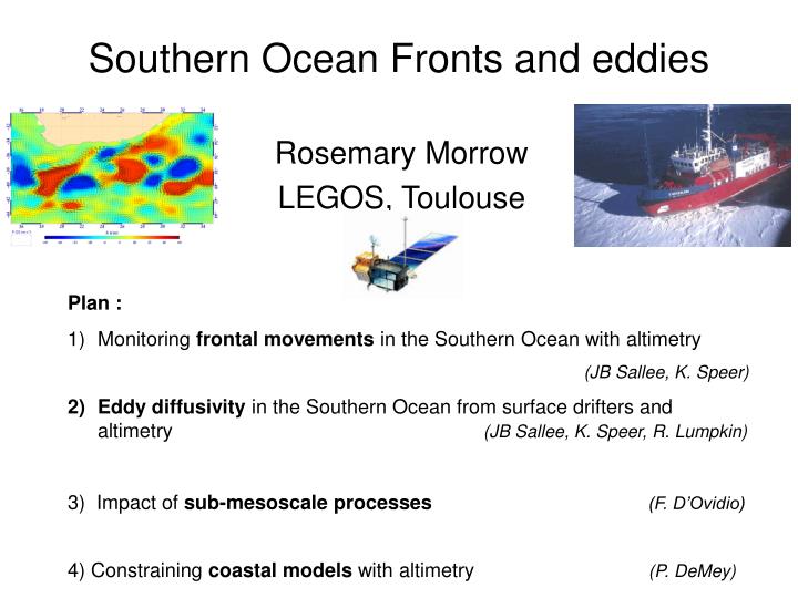
Southern Ocean Fronts and eddies • Plan : • Monitoring frontal movements in the Southern Ocean with altimetry • (JB Sallee, K. Speer) • Eddy diffusivity in the Southern Ocean from surface drifters and altimetry (JB Sallee, K. Speer, R. Lumpkin) • 3) Impact of sub-mesoscale processes(F. D’Ovidio) • 4) Constraining coastal models with altimetry (P. DeMey) Rosemary Morrow LEGOS, Toulouse
1. Fronts Fronts are generally described by horizontal property gradients (T, S, O2, N2, Dyn ht, etc), either at the surface or subsurface Dyn height ( altimetry) – SR3 Section Neutral Density – SR3 Section Tasmania Antarctica Fronts detected in September 1996 – SR3 – between Tasmania and Antarctica Sokolov and Rintoul, 2004
Detecting Southern ocean fronts Monitor front movements using absolute SL Strong SLA gradients often peak at absolute sea level contours ASL = (SLA + mean sea surface) => Gradient of sea surface height for January 1995 SR3 (color), with selected height contours corresponding to particular fronts Jets merge and split, strengthen and weaken. (Sokolov and Rintoul, JMS, 2002; JPO, 2006). => Southern Ocean fronts are deep-reaching – can monitor their movements using altimetric absolute sea level
Variability of Southern Ocean frontsi) Topographic influence along the circumpolar belt 3. Variabilité frontale Frequency of SAF occurrence Variabilité du SAF SAF Variability: Mean position +/- 1 STD Red = low variability Fronts remain ~fixed Blue = strong variability : Fronts move over a large area Intensity (dh/dy) Does atmospheric variability impact on the frontal positions in deep basins ? Sallée et al. - Response of the ACC to atmospheric variability – J. Clim (2008)
3. Variabilité frontale Variability of the frontsii) Response to the climate variability : SAM and ENSO Atmosphere Ocean SLP/SAM SLA/SAM SLP/ENSO SLA/ENSO Sallée et al. - Response of the ACC to atmospheric variability - – J. Clim (2008)
Variability of the frontsii) Response to the climate variability : SAM and ENSO Covariance of PF and SAM or ENSO SE Pac Indian High frequency : (<3 month) SAM dominates Low frequency : (>1 year) ENSO dominates
Variability of the frontsiii) Mechanisms controlling the variability Meridional Ekman transport anomaly regressed onto SAM : Indian Ocean : Max Ekman transport SOUTH of the fronts Response to a positive SAM event (timescale ~2 weeks) V ekman Sallée et al. - Response of the ACC to atmospheric variability -
Variability of the frontsiii) Mechanisms controlling the variability SE Pacific basin : Max Ekman transport NORTH of fronts Response to a positive SAM event (timescale ~2 weeks) V ekman Sallée et al. - Response of the ACC to atmospheric variability -
Fronts – future with SWOT - Altimetry is important for monitoring subsurface frontal movements • Currently using gridded AVISO maps (limited by the optimal interpolation scales : spatial : 70-100 km at mid to high latitude, temporal : 15-20 days) • Hydrographic Fronts will have geostrophic adjustment at surface • Need to resolve the Rossby radius : • 10-20 km at high latitude • > 3-5 days • => Measurements every 3-5 km
Eddy Diffusion and the Southern Oceanmixed layer heat budget 2. J.B. Sallee, K. Speer, R. Morrow, R. Lumpkin (JMR submitted, 2008)
Calculating Eddy Diffusion Effective Diffusivity (Taylor, 1921) : In well-sampled homogeneous turbulence, k ~ constant after several integral time-scales T is the Lagrangian timescale, related to the velocity autocorrelation function, R : Frequently studied in theory. In practice, we need lots of lagrangian particules.
Calculating Lagrangian timescale (T), and velocity ACF, (R)from Global Drifter Program (GDP) 1995-2005and virtual drifters from altimetric currents 10 years of lagrangian drifter data Snapshot of altimetric currents overlaid on SLA Observed cross stream dispersion around the ACC from lagrangian GDP drifters Linear dispersion regime
Cross stream eddy scales from GDP drifters Lagrangian eddy time-scales first zero crossing (days) Lagrangian eddy space-scales (km) Eddy diffusion and the Upper Cell of the Southern Ocean
Cross stream eddy diffusion (Sallee et al., 2008) • Statistics calculated from GDP surface drifters in Southern Ocean. • higher around ACC and in western boundary currents 1-2 x 10⁴ – order of magnitude larger than applied in climate models
Alongstream averages : Contribution and Error PF SAF SAF-N Particles on drifter “grid” Real Drifters 0.5 deg grid particles Without WBCs Ekman Mesoscale geostrophic eddy contribution dominates. Ekman contribution is weak. Higher values than previous Southern Ocean studies. - Consistent values with Gulf Stream or Kurushio calculations from GDP drifters. – Sallee and Speer - jbsallee@gmail.com
Application : Eddy heat diffusion Eddy heat diffusion in W.m-2 Winter mixed layer depths (m) Here, eddy heat diffusion in the mixed layer is : Temperature gradient derived from TMI/AMSR satellite SST data Impact on the formation of deep winter mixed layers in the Southern Ocean (Sallee et al; GRL, 2007) Eddy diffusion and the Upper Cell of the Southern Ocean
Eddy heat fluxes around Kerguelen Annual mean eddy heat diffusion SAZ STF SAZ SAF -10 0 10 W.m-3 Eddy diffusion coefficient estimated from GDP drifters (Davis, 1991), and meridional SST gradient is from satellite TMI/AMSR T-S Diagram of a composite of ARGO floats in the SAZ Strong « interleaving » near Kerguelen – cooling and freshening from eddy mixing Sallee et al. 2006, Ocean Dynamics
Summary – Eddy Diffusion Surface Drifters and altimetry -> similar estimation in situ and satellite of eddy diffusion Linear dispersion regime dominated by geostrophic mesoscale eddies Values order 104 m2.s-1 in the western boundary current regions Need to resolve Rossby radius
Submesoscale Eddies 3. R. Morrow, F. D’Ovidio, A. Koch-Larrouy, J.B. Sallee (Jason-II CNES/NASA Proposal)
Submesoscale Eddies Estimating sub-mesoscale circulation from ¼° AVISO velocity maps ALTIMETRIC EULERIAN FIELD • Simple, instantaneous description • Mesoscale structures O(100 km) • 2D maps of horizontal currents used to estimate lagrangian evolution of filaments O (10 km) LAGRANGIAN MANIFOLDS (FSLE) • Time-integrated structures • Precise localization of transport barriers and filaments • Strong mixing in submesoscale structures With F. D’Ovidio, LMD
Traditional analysis : altimetric EKE Mesoscale eddies Resolution 30 km 5 dec. 2000 Lagrangian analysis (Lyap. Exp) Sub-mesoscale Filaments Resolution 1-10 km 5 dec. 2000
DIMES campaign: • => release Lagrangian floats close to altimetry-detected hyperbolic points, to : • "compute" in-situ the Lyapunov exponents • follow the unstable manifolds, that for short times (a week or so) can be approximated by nearby lagrangian trajectories. • The length of the unstable manifold can be related to eddy diffusion, within the formalism of the effective diffusivity. • Emily Shuckburg (BAS), Francesco d’Ovidio (LMD)
Constraining coastal ocean models with altimetry Pierre De Mey, LEGOS/POC WATER-HM/SWOT meeting CNES HQ, Paris, February 2008
Non-local, structured errors in coastal current SLA Depth-averaged velocity Surface salinity Temperature EOF-1 79.8 % What is this? Ensemble multivariate EOFs in the Catalan Sea coastal current in response to coastal current inflow perturbations (mimicking downscaling errors). Relevance to WATER-HM? SLA errors are small-scale (O(40km)) and strongly correlated to fine-scale (u,v,T,S) 3-dimensional errors which we can then expect to correct if SLA is observed at sufficiently fine scales. EOF-2 11.0 % EOF-3 4.9 % (Jordà et al., 2006)
Non-local, structured errors in coastal current SLA Depth-averaged velocity Surface salinity Temperature EOF-1 79.8 % EOF-2 11.0 % EOF-3 4.9 % (Jordà et al., 2006)
Activation of coherent error features by storms What is this? The SLA component of a particular ensemble EOF in response to atmospheric forcing errors. It is a proxy of the actual model errors. As the time series shows, it is activated during the July 7-8 storm and is characterized by a shelf-wide response, a surge response, and a mesoscale response with O(1day) time scale. Relevance to WATER-HM? Questions 1 (mesoscale), 2 (coastal) and 3 (storm-related). We expect a wide-swath altimeter to consistently constrain the fine-scale, multivariate ocean response to those fast events, and hopefully help better predict the associated phenomena. Ensemble EOF-3 SLA, 3D BoB model A B July 1 2004 August 31
Time variations of ensemble variance Point A: EC Point B: BoB SLA, Ub errors linked to local wind errors Kelvin waves propagation in error subspace SLA errors attributable to pressure errors
Wide-swath vs. nadir in Bay of BiscayStochastic modelling with atm. forcing perturbations in 3D BoB (left panel) What is this? The RM spectra plot on the left shows the number of degrees of freedom of model (forecast) error which can be detected by a particular array amidst observational noise. This is done by counting eigenvalues above 1. This is shown for three arrays (legend). Representer matrices are calculated by stochastic modelling with atmospheric forcing errors. Relevance to WATER-HM? Questions 1 (mesoscale) and 2 (coastal). One Wide-Swath altimeter on a JASON orbit detects 4 degrees of freedom, while one nadir instrument (JASON) detects only one. The more d.o.f.’s are detected, the more critical ocean processes will be constrained. Array Modes -- SLA Scaled RM spectra Top: Wide Swath (4 dof’s) Mid: WS over deep ocean (2 dof’s) Bottom: JASON (1 dof) “Slosh” Meso1 Meso2 (after Le Hénaff & De Mey, 2008)
(right panel) What is this? The “array modes” of model error corresponding to the spectra to the left. For each array, mode 1 is mostly water sloshing around between shelf and deep-ocean domains; modes 2 and 3 are a mix of mesoscale & submeso response, slope current variability and shelf processes. Relevance to WATER-HM? Questions 1 (mesoscale) and 2 (coastal). As was seen on the left panel, JASON can only detect (and constrain) the “slosh” mode. One needs a wide-swath instrument to detect (constrain) all three modes + a 4th one not shown. In this way, one can objectively demonstrate that a wide-swath instrument is needed to constrain the coastal ocean mesoscale and coastal current variability. (A collaboration between LEGOS and OSU’s OST proposals has been proposed on this topic) Wide-swath vs. nadir in Bay of BiscayStochastic modelling with atm. forcing perturbations in 3D BoB Array Modes -- SLA Scaled RM spectra Top: Wide Swath (4 dof’s) Mid: WS on deep ocean (2 dof’s) Bottom: JASON (1 dof) “Slosh” Meso1 Meso2 (after Le Hénaff & De Mey, 2008)
Summary – what is needed : SWOT • Space : Resolving the Rossby radius in the Southern Ocean : 10-20 km means sea level observations at 2-5 km • Time : Resolving geostrophic adjustion time-scales of 2-5 days =>With this resolution, finer scale filaments can be determined (eg FSLEs) • Precision : cms
Impact of internal tides Regions of conversion of M2 barotropic tide into baroclinic internal waves Le Provost et al. 1994, Lyard et al., 2006 Parametrisations exist for this conversion : - 1/3 energy dissipated locally with bottom drag - 2/3 energy radiates away as internal tides In small closed seas or basins, internal tides also dissipate locally
I. ITF - 1) Parametrisation of tidal mixing in ¼° OGCM Koch-Larrouy et al. 2007
Impact of the internal tides on coupled ocean-atmosphere models SST Koch-Larrouy et al. 2008
Jason-II proposal : Submesoscale Eddies and Tidal mixing 1) Analyse the role of eddy fluxes and tidal mixing in modifying SAMW and AAIW in key regions, using the DRAKKAR ¼° model (Ariane Koch-Larrouy, Post-Doc, LEGOS, 2008) Winter ML density, ML > 300 m, (Sallee et al. 2007) Kerguelen Macquarie Ridge Fracture Zone Drake Passage M2 internal tide generation sites, (Le Provost et al. 1994, Carrère et Lyard 2003)
Monitoring fronts with satellite data :Meridional gradients in SSH and SST Grad SSH : Surface position can be offset from subsurface position Eg. Summer stratification + strong Ekman transport can shift surface fronts northward in summer SSS data Grad SST : Altimetry is important for monitoring subsurface frontal movements
Winter ML heat budget terms Air-sea Flux, Q Ekman Heat Flux Zones clés Eddy heat flux Total : 3 terms Sallee et al. 2007, GRL
Winter ML heat budget terms Winter ML depth Total heat forcing : 3 terms
Circumpolar evolution of winter ML Sum of 3 forcing terms in winter – relative to the SAF-N axis Winter ML Depth – relative to the SAF-N axis Winter ML Density for ML > 200 m