Download

1 / 19
190 likes | 270 Views
A Random Coefficient Model Example: Observations Nested Within Individuals. Academy of Management, 2010 Montreal, Canada Jeffrey B. Vancouver Ohio University. Within-Person Level of Analysis. Longitudinal Models Growth curve modeling Time series Repeated-measures

E N D
A Random Coefficient Model Example: Observations Nested Within Individuals Academy of Management, 2010 Montreal, Canada Jeffrey B. Vancouver Ohio University
Within-Person Level of Analysis • Longitudinal Models • Growth curve modeling • Time series • Repeated-measures • Multiple decisions, tasks, etc. • Where, time is often a nuisance variable (practice/fatigue effects) to be controlled • Lagged effects models
Sample Phenomena • Dynamic criteria • Learning • Socialization • Treatment/intervention evaluation • Stress, attitude, turnover research Predicting slopes and intercepts Testing causal hypotheses
Training Effects Example • Finding best-fitting trajectory by ignoring individual violates independence of observation assumption • More importantly, • Might want to find out what determines • Intercept • Slope • E.g., • Training (e.g., self-paced training for new Plant A employees) • Individual differences (predictor scores)
COG COG COG COG COG COG COG 150 150 150 150 150 150 150 125 125 125 125 125 125 125 100 100 100 100 100 100 100 75 75 75 75 75 75 75 50 50 50 50 50 50 50 1 1.5 2 1 1 1 1.5 1.5 1.5 2 2 2 1 1.5 2 1 1 1.5 1.5 2 2 AGE AGE AGE Individual Trajectories Performance High low 0 1 2 3 4 5 6 7 Time (months)
Unconditional Models • Unconditional (null) Means model • L1: y = π0 + e • L2: π0 = β00 + r • Unconditional growth model • L1: y = π0 + π1 time + e • L2: π0 = β00 + r π1 = β10 + r Note changes in notation (pi, e for within-person)
Conditional Models • Conditional growth model • L1: y = π0 + π1 time + e • L2: π0 = β00 + β01 TRAIN + β02 COGA + r π1 = β10 + β11 TRAIN + β11 COGA + r Dummy code for in training group (1) or not (0) cognitive ability score
HLM Output The outcome variable is PERFORM The model specified for the fixed effects was: ---------------------------------------------------- Level-1 Level-2 Coefficients Predictors ---------------------- --------------- INTRCPT1, P0 INTRCPT2, B00 TRAIN, B01 COGA, B02 TIME slope, P1 INTRCPT2, B10 TRAIN, B11 COGA, B12 Summary of the model specified (in equation format) --------------------------------------------------- Level-1 Model Y = P0 + P1*(TIME) + E Level-2 Model P0 = B00 + B01*(TRAIN) + B02*(COGA) + R0 P1 = B10 + B11*(TRAIN) + B12*(COGA) + R1
Fixed Effects Output The outcome variable is PERFORM Final estimation of fixed effects (with robust standard errors) ---------------------------------------------------------------------------- Standard Approx. Fixed Effect Coefficient Error T-ratio d.f. P-value ---------------------------------------------------------------------------- For INTRCPT1, P0 INTRCPT2, B00 4.252554 0.056756 74.926 129 0.000 TRAIN, B01 -0.684429 0.080463 -8.506 129 0.000 COGA, B02 0.019250 0.116900 0.165 129 0.870 For TIME slope, P1 INTRCPT2, B10 0.191658 0.012714 15.075 129 0.000 TRAIN, B11 0.045514 0.019159 2.332 129 0.005 COGA, B12 0.038086 0.021712 1.754 129 0.081 ----------------------------------------------------------------------------
Fixed Effects Output(re “centered” time) The outcome variable is PERFORM Final estimation of fixed effects (with robust standard errors) ---------------------------------------------------------------------------- Standard Approx. Fixed Effect Coefficient Error T-ratio d.f. P-value ---------------------------------------------------------------------------- For INTRCPT1, P0 INTRCPT2, B00 4.252554 0.056756 74.926 129 0.000 TRAIN, B01 0.264429 0.090463 3.506 129 0.000 COGA, B02 0.019250 0.116900 0.165 129 0.870 For TIME slope, P1 INTRCPT2, B10 0.191658 0.012714 15.075 129 0.000 TRAIN, B11 0.025514 0.019159 1.332 129 0.185 COGA, B12 0.038086 0.021712 1.754 129 0.081 ----------------------------------------------------------------------------
Interpretationsa • Training group • Groups were not equivalent on performance initially • Training effect made up for initial deficit (-.68) and then some (+.26). • Cognitive ability (g) • Not much of a player; only marginally predicted growth in performance over time • Might be useful to test interaction of training condition and g to see if g led to faster improvement for training group aCaveat: this is a made up example
Random Effects Output Final estimation of variance components: ----------------------------------------------------------------------------- Random Effect Standard Variance df Chi-square P-value Deviation Component ----------------------------------------------------------------------------- INTRCPT1, R0 0.46142 0.21291 129 4451.18764 0.000 TIME slope, R1 0.06074 0.00369 129 220.46760 0.000 level-1, E 0.50582 0.25585 ----------------------------------------------------------------------------- Statistics for current covariance components model -------------------------------------------------- Deviance = 4758.579866 Number of estimated parameters = 4
Time Series (internally valid designs) • Interrupted: • O OOOO X O OOOO • Control series • O OOO X O OOOOOO O OO • O OOOOOOOOOO X O OO • Non-equivalent dependent variables • OAOAOAOA X OAOAOA • OBOBOBOB X OBOBOB • Removal • O OO X O OOOX O OO Switching Replications (bringing waitlisted on-line)
π0= β00+ β01z + u π1= β10+ β11z + u π2= β20+ β21z + u π3= β30+ β31z + u Examining Effect of Interventions/Events Using HLM Level 2: individual z = 1 if in treatment/exposed to event 0 if control/not exposed t = 0 1 2 3 4 5 6 7 8 9 . . . k d = 0 0 0 0 0 1 1 1 1 1 1 1 1 d = 0 0 0 0 0 1 2 3 4 5 6 7 8 t-k = . . . . . . . . . -5 -4 -3 -2 -1 0 y = π0+ π1t + π2d + π3td + e y = outcome t = time d = dummy Level 1: occasion (within person)
Other issues • Nonlinear effects • Growth CURVE implies time effects are not linear • Adding polynomials (e.g., time2; time3) provides simple, preliminary (and often final) test for curves • Singer & Willett (2003) Applied Longitudinal Data Analysis • Graph results • Plug variable values into equations, minding centering decisions • Helpful to self and audience • Dichotomous DVs (e.g., choice) • Bernoulli distribution available in HLM (output includes odds ratios) • E.g., in Vancouver, More, & Yoder (2008) JAP • Examining relationships among time-varying variables using lagged RCM, manipulations • E.g., Vancouver, Thompson, Tischner, & Putka (2002) JAP
Q & A Dave Hofmann Mark Gavin Jeff Vancouver
Predicting Effects of Time-Varying Passively Observed Variables • If X and Y are measured simultaneously, reciprocal and 3rd variable effects confound interpretations • Lagged RCM can test reciprocal issue: • provided lags are properly specified • provided trend effects controlled (only issue if reciprocity) • Control for time • Control for y(t-1) • 3rd variable problem still possible
Or more generally: Yij = π0j + π1j(Xij) + rij Lagged RCM Time Individual 1 2 3 4 x x x x A YtA = πAX(t - 1)A y y y x x x x B YtB = πBX(t - 1)B y y y : : : : : : x x x x Ytj = πjX(t – 1)j n y y y