Chapter 10 PID Controls

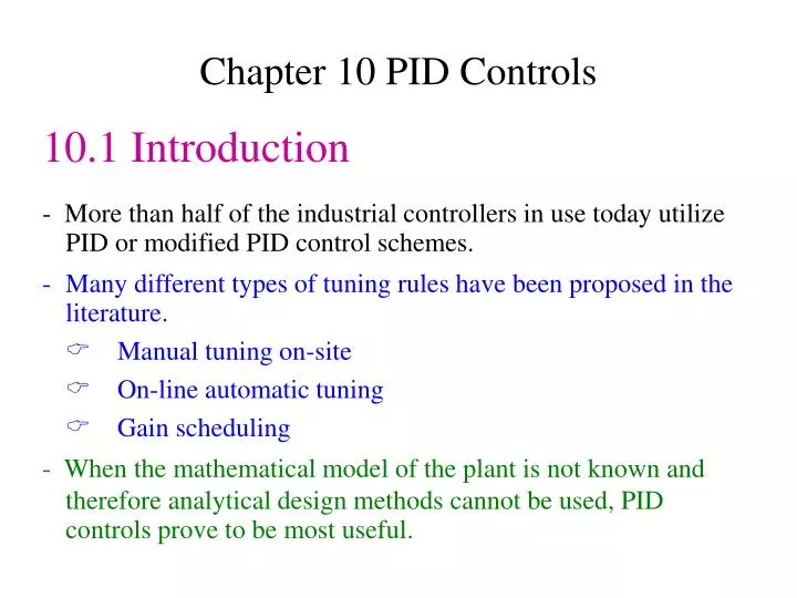
1. Chapter 10 PID Controls 10.1 Introduction - More than half of the industrial controllers in use today utilize PID or modified PID control schemes. • Many different types of tuning rules have been proposed in the literature.  Manual tuning on-site  On-line automatic tuning  Gain scheduling - When the mathematical model of the plant is not known and therefore analytical design methods cannot be used, PID controls prove to be most useful.

2. Figure 10-1 PID control of a plant. Design PID control - Know mathematical model  various design techniques - Plant is complicated, can’t obtain mathematical model experimental approaches to the tuning of PID controllers

3. Ziegler-Nichols Rules for Tuning PID Controllers • Ziegler and Nichols proposed rules for determining values of the proportional gain Kp, integral time Ti,and derivative time Tdbased on the transient response characteristics of a given plant. • Such determination of the parameters of PID controllers or tuning of PID controllers can be made by engineers on-site by experiments on the plant. • Such rules suggest a set of values of Kp,Ti,and Tdthat will give a stable operation of the system. However, the resulting system may exhibit a large maximum overshoot in the step response, which is unacceptable. - We need series of fine tunings until an acceptable result is obtained.

4. Ziegler-Nichols 1st Method of Tuning Rule - We obtain experimentally the response of the plant to a unit-step input, as shown in Figure 10-2. • The plant involves neither integrator(s) nor dominant complex-conjugate poles. • This method applies if the response to a step input exhibits an S-shaped curve. - Such step-response curves may be generated experimentally or from a dynamic simulation of the plant. Figure 10-2 Unit-step response of a plant.

5. L = delay time T = time constant Figure 10-3 S-shaped response curve.

6. Transfer function: Table 8-1 Ziegler–Nichols Tuning Rule Based on Step Response of Plant (First Method)

8. Ziegler-Nichols 2nd Method of Tuning Rule 1. We first set Ti= and Td = 0. Using the proportional control action only (see Figure 10-4). Figure 10-4 Closed-loop system with a proportional controller.

9. 2. Increase Kpfrom 0 to a critical value Kcrat which the output first exhibits sustained oscillations. Figure 8-5 Sustained oscillation with period Pcr.(Pcr is measured in sec.)

10. Ziegler and Nichols suggested that we set the values ofvthe parameters K,, T,, and Td according to the formula shown in Table 10-2. Table 10-2 Ziegler–Nichols Tuning Rule Based on Critical Gain Kcr and Critical Period Pcr (Second Method)

12. Figure 10-6 PID-controlled system.

15. Figure 10-7 Block diagram of the system with PID controller designed by use of the Ziegler–Nichols tuning rule (second method).

17. Figure 10-8 Unit-step response curve of PID-controlled system designed by use of the Ziegler–Nichols tuning rule (second method).

18. The maximum overshoot in the unit-step response is approximately 62%.The amount of maximum overshoot is excessive. It can be reduced by fine tuning the controller parameters. Such fine tuning can be made on the computer. We find that by keeping Kp= 18 and by moving the double zero of the PID controller to s= -0.65, that is, using the PID controller See Figure 10-9

19. Figure 10-9 Unit-step response of the system shown in Figure 8–6 with PID controller having parameters Kp = 18, Ti = 3.077, and Td = 0.7692.

22. - Varying the value of K (from 6 to 30) will not change the damping ratio of the dominant closed-loop poles very much. Figure 10-11 Root-locus diagram of system when PID controller has double zero at s = –1.4235.

23. Figure 10-12 Root-locus diagram of system when PID controller has double zero at s = –0.65. K = 13.846 corresponds to Gc(s) given by Equation (10–1) and K = 30.322 corresponds to Gc(s) given by Equation (10–2).

24. Figure 10-13 PID-controlled system.