Download
1 / 35
360 likes | 560 Views
SIGNIFICANT SOIL PROPERTIES. M. Zoghi, Ph.D., P.E. Geotechnical Design Fall 2008. OUTLINE. Overview Permeability & Seepage Compressibility & Settlement Shear Strength Examples. II. Permeability and Seepage. Bernoulli’s Theorem Darcy’s Law Coefficient of Permeability

E N D
SIGNIFICANT SOIL PROPERTIES M. Zoghi, Ph.D., P.E. Geotechnical Design Fall 2008
OUTLINE Overview Permeability & Seepage Compressibility & Settlement Shear Strength Examples
II. Permeability and Seepage • Bernoulli’s Theorem • Darcy’s Law • Coefficient of Permeability • Flow Net Construction • Seepage Quantity • Uplift Pressure • Drainage • Geosynthetics
Bernoulli’s Theorem u = p = fluid pressure at any point in the body of water Total Head, h = Pressure Head (u/w) + Elevation Head (Z) + 0 Hydraulic gradient, i = h / L Das, 2001
Darcy’s Law V = k i Das, 2001
Coefficient of Permeability • Units: • Ft/min., ft/day, cm/sec, etc. • Factors: • Grain-size dist., void ratio, fluid viscosity, etc. • Typical Values • Empirical Relationships: • Hazen’s Formula: K(mm/sec) = C D10 Typical Values Soil Type k (cm/sec) Clean Gravel 100-1 Coarse Sand 1.0-0.01 Fine Sand 0.01-0.001 Silty Clay 0.001-0.00001 Clay0.000001 2 C = 10 D10= Effective Size, mm
Lab Tests K = Q L / (Aht) Constant Head Test Das, 2001
Falling Head Test K = 2.303 (aL/At) log (h1/h2)
Draw-Down Field Tests 2 2 K = [2.303 q log (r1/r2)] / [ (h1 – h2) Das, 2001
Elements of Flow Net Theory General • A set of flow lines and equip. lines • A flow line – along which a water particle travels • An equip. line – joining pts with the same piezometric elevations (i.e., hydraulic head) Step-by-Step(Trial Sketching) • Draw the hydraulic structure to a convenient scale • Establish the boundary flow & equip. lines • No more than 3 – 5 flow channels • Examine the flow net for being both perpendicular & pseudo-square
Example U = (Total Head – Elev. Head)w McCarthy, 2002
Drainage • Rule of Thumb: if k≥5 X 10^(-5) mm/sec then cont. drainage required! • Dewatering Shallow Excavations - interceptor ditches and sump pits • Dewatering Intermediate Depths – well points (single/multistage), vacuum dewatering system, elctro-osmosis • Deep Drainage – deep wells and deep well pumps • Consolidation Drainage – surcharge application, use of sand drains, and wick drains • Drainage After Construction – foundation drains, blanket drains, interceptor drains
Geosynthetics • Synthetic Fabrics • Separation • Filtration • Drainage • Reinforcement • Barriers or containment • Protection • Erosion control
Stress Distribution Within Soil Mass Boussinesq Theory 0 0 Circular Area
III. Compressibility & Settlement • Fundamental Concepts • One-Dimensional Consolidation Theory • Load-Deformation Characteristics • Consolidation Characteristics • Stress Distribution • Amount of Consolidation • Time-Rate of Consolidation Said Big Ben to Leaning Tower of Pisa: " If you have the inclination, I have the time ..."
Soil Profile Spring Analogy Lamb & Whitman, 1969 Das, 2001
Laboratory Test Das, 2001
Components of Settlement St= Spc+ Ssc+ Svd St= Total Settlement Spc= Primary Consolidation Settlement Ssc= Secondary Consolidation Settlement Svd= Distortion (immediate) settlement Das, 2001
Typical e-log p curve Virgin Curve Rebound Curve Unloading Curve Recompression Curve Das, 2001
Casagrande’s Method of Finding Preconsolidation Stress Cc Cc = 0.009(LL – 10)
Components of Consolidation Settlement Normally Consolidated Soils: Spc= [Cc/(1+e0)] H0log [(’0 + )/ ’0] where: vf = (’o + ) Overconsolidated Soils:(OCR = ’c /’0) Spc= [Cr/(1+e0)]Holog [(’0 + )/ ’0] for (’0 + ) ’c Spc= [Cr/(1+e0)]Holog (’c /’0) + [Cr/(1+e0)] H0log [(’0 + )/ ’c] for (’0 + ) ’c Secondary Consolidation: Ssc= [C/(1+eo)]Holog (tf/tp) Cr= 1/5 to 1/10 of Cc C = (0.03 to 0.06) Cc
Time-Rate of Consolidation Cv = Tv H2dr / t Das, 2001
IV. Shear Strength Coduto, 1999
Block Analogy • Attributed to three basic components: • Frictional resistance to sliding between solid particles • Cohesion and adhesion between soil particles • Interlocking and bridging of solid particles to resist deformation Coduto, 1999
Mohr-Coulomb Failure Criterion = c + ’ tan Das, 2001
Direct Shear Test Das, 2001
Triaxial Compression Test Das, 2001
Unconfined Compression Test Das, 2001