Download
1 / 33
330 likes | 485 Views
Computability. Chapter 5. Overview. Turing Machine (TM) considered to be the most general computational model that can be devised ( Church-Turing thesis ) TMs are a litmus test for computational feasibility – If a task can be done on a Turing machine, it is feasible

E N D
Computability Chapter 5
Overview • Turing Machine (TM) considered to be the most general computational model that can be devised (Church-Turing thesis) • TMs are a litmus test for computational feasibility – • If a task can be done on a Turing machine, it is feasible • If it cannot, it is considered infeasible • There are well-defined tasks, notwithstanding, that cannot be done on a TM • Different flavors of TM have been devised • Multi-tape, multi-head TMs • Nondeterministic TMs • All can be shown to be equally powerful vis-à-vis feasibility • Universal TM can be defined
The Standard Turing Machine Model (cont.) • Two modes of TM use vis-à-vis languages:
0,R 1,R q1 h , Start Programming the Turing Machine • Programs can be expressed as a functional table: • Or as a transition diagram:
And as a transition diagram: 1,R ,0 q4 0,R ,R q2 h 0,0 , 1,0 0, ,1 0,1 q5 1,1 q1 ,R 1,R q3 0,R 1, Start Programming the Turing Machine (cont.) • Another program expressed as a functional table:
Extensions to the StandardTuring Machine Model • Double-ended tape Turing machine: tape is of indefinite length on both sides
Tape Unit ControlUnit Extensions to the StandardTuring Machine Model (cont.) • Can be simulated by a standard TM whose one, single-ended tape has two tracks: upper track recording right half of the double-ended tape and lower track recording left half
Tape Unit ControlUnit Extensions to the StandardTuring Machine Model (cont.) THEOREM 5.2.0 For each double-ended Turing machine Mdthere is a standard Turing machine M such that a terminating T-step computation by Mdcan be simulated in O(T2) steps by M. • Proof (sketch): Simulate each move of the double-ended tape TM Mdon a standard TM M by • scanning the tape to determine the position of and symbol scanned by the head of the double-ended TM MdO(T); and then • simulating the operation to mimic what Mdwould do O(1)
Extensions to the StandardTuring Machine Model (cont.) • k-tape Turing machine: one control unit and k single-ended tapes of indefinite length
ControlUnit Extensions to the StandardTuring Machine Model (cont.) • k-tape Turing machine: can be simulated by a standard Turing machine whose one tape has k tracks and a large tape alphabet
ControlUnit Extensions to the StandardTuring Machine Model (cont.) • Proof (sketch): Simulate each move of the k-tape TM on the standard TM by • scanning its single tape and collecting information that the control unit of the k-tape TM would “know” from each of its k tape heads O(T); and then • simulating the move of the k-tape TM by altering its single tape at the appropriate cell O(T)
1,1 1,R Start Extensions to the StandardTuring Machine Model (cont.) • Proof (sketch): Simulate the moves of the nondeterministic TM MND on input w with a standard TM MD by using three tapes • one tape is read-only and contains the input w which is never altered; • another tape is a “work tape” which is used to simulate MND • yet another tape contains the current “guess” or sequence of choices used in simulating MND
xj1 xj+1 xn x1 x2 xj p state Configuration Graphs • configuration allows for “reconstruction” of TM and its current state from a string representation
h1 x1 h2 p x2 state hk xk Configuration Graphs (cont.) • configuration allows for “reconstruction” of the k-tape TM and its current state from a string representation
final stateconfiguration initial stateconfiguration Configuration Graphs (cont.)
Sample derivation SaSBCaaBCBCaaBBCC aabBCC aabbCC aabbcC aabbcc (c) (d) (a) (b) (g) (f) (e) Phrase-Structure Languagesand Turing Machines (cont.) • Language generated by this grammar is L(G) = {anbncn|n1}
[sw1w2…wn] Configuration graph of TM acceptance of w [h1] Phrase-Structure Languagesand Turing Machines (cont.) • Proof: Design a phrase-structure grammar that would capture the (d)evolution of the acceptance of a string w by a TM. • starting with the acceptance configuration of [h1], grammar rules will allow us to trace backwards towards the start configuration of [sw1w2…wn] • yet other grammar rules will then strip extraneous symbols such that only the string w1w2…wn remains • establish that any string w accepted by some TM can be generated by a phrase-structure grammar establishing the theorem S [h1] … [sw1w2…wn] …w1w2…wn
Phrase-Structure Languagesand Turing Machines (cont.) • Proof: Design a phrase-structure grammar that would capture the (d)evolution of the acceptance of a string w by a TM. • Let deterministic TM be M = (,Q,,s,h) • The desired grammar G = (N,T,R,s) is such that N =Q{s,,[,]} T = and the grammar rules are:
w input tape Control Unit w’ work tape Phrase-Structure Languagesand Turing Machines (cont.) • Proof: Design a TM that would accept a string w if it is possible to generate it with the production rules of a phrase-structure grammar G and “hang” when it isn’t possible to do so • TM will be a 2-tape nondeterministic TM • One tape will hold the candidate string w; the other will be a “work” tape • TM nondeterministically simulates the production of string w’ by the phrase-structure grammar G on the work tape • If no production produces w, TM enters into an infinite loop
Universal Turing Machines • allows for the complete and accurate definition and description of a standard TM with a string
1,R ,0 q4 0,R ,R q2 h 0,0 , 1,0 0, ,1 0,1 q5 1,1 q1 ,R 1,R q3 0,R 1, Start Universal Turing Machines (cont.) • Previous example would be encoded canonically as:
w work tape Control Unit (M) program tape Universal Turing Machines (cont.) • A Universal Turing Machine (UTM) is capable of simulating an arbitrary Turing Machine M on an arbitrary input word w. • One possible UTM is a two-tape TM that may be described as: • One tape is a work tape, starts out as containing w; • Second tape is the program tape, starts out as containing (M), the canonical encoding of M • Tape symbol alphabet is:
w work tape Control Unit (M) program tape Universal Turing Machines (cont.) • A Universal Turing Machine (UTM) is capable of simulating an arbitrary Turing Machine M on an arbitrary input word w. • One possible UTM is a two-tape TM that may be described as: • The UTM simulates M by locating on the program tape the appropriate transition given the current state of M and the symbol on the work tape being scanned by its head • When the transition is located, the UTM carries out the operation on the work tape • There is a standard UTM equivalent to this two-tape UTM
TM Generator j (Mj) Encoding of Strings and Turing Machines • Any set of strings can be arranged in lexicographic order based on the “order” of the symbols as listed in its alphabet set = {,,} S: {,,,,} S’: {,,,,} • Turing machines can be listed in lexicographic order based on the “order” of their canonical encodings (strings over some alphabet) • Generating the jth Turing machine can be mechanized
A language L is recursively enumerable if there is a TM that accepts just the strings of L, possibly not halting on strings not in L. Limits on Language Acceptance • A language L is decidable(or recursive) if there is a TM that halts on all inputs and accepts just the strings of L • A language L is unsolvable if it is recursively enumerable but not decidable
Limits on Language Acceptance (cont.) • The following results identify three languages that are decidable: • The following result identifies a language that is notrecursively enumerable: • Proof: By contradiction and use of diagonalization.
Limits on Language Acceptance (cont.) • The following results identify a language that is unsolvable (i.e., recursively enumerable but notdecidable): • Proof: Reclassify states, switching accepting and non-accepting. • Proof: Using a Universal Turing machine, run Miwith input wi. This shows the language is recursively enumerable. Since its complement is not recursively enumerable, therefore not decidable, it cannot be itself decidable.
A (solves L) R (translates L to A) input to L input to A output Algorithm for L Reducibility andUnsolvability • Use the “traditional” technique of reduction to establish that other languages are unsolvable: • By contradiction:assume that an algorithm A exists for candidate language L then show we can use A to obtain an algorithm for a language previously known as unsolvable
Reducibility andUnsolvability (cont.) • Existence of such a “reducing algorithm” means one can mechanize the acceptance of one language by using the mechanism of accepting the other language:
A (solves L2) R (translates L1 to L2) input to L1 input to L2 output “Algorithm” for L1 Reducibility andUnsolvability (cont.) • This lemma is useful in arriving at unsolvability results:
Reducibility andUnsolvability (cont.) • Use this reducibility lemma to establish that the following language is unsolvable(i.e., recursively enumerable but not decidable): • Proof: Use encoding of M and w as input to universal Turing machine and simulate M with w as input. This establishes recursive enumerability. Use Lemma 5.8.1 to establish non-decidability by reducing L1 to LH . The “reducing algorithm” generates the ith input string and the ith Turing machine and uses those as input to “imaginary” machine deciding LH and then “reverses” the polarity of the output. This decides L1.