Download
1 / 72
720 likes | 959 Views
Abstractions and Decision Procedures for Effective Software Model Checking. Prof. Natasha Sharygina The University of Lugano, Carnegie Mellon University. Microsoft Summer School, Moscow, July 2011 Lecture 1. Outline . Day 1 ( Lectures 1 and 2) Model Checking in a Nutshell

E N D
Abstractions and Decision Procedures for EffectiveSoftware Model Checking Prof. Natasha Sharygina The Universityof Lugano, Carnegie Mellon University Microsoft Summer School, Moscow, July 2011 Lecture1
Outline • Day 1 (Lectures 1 and 2) • ModelCheckingin a Nutshell • Abstractions in ModelChecking • Predicate Abstraction • SAT-based approach
Guess what this is! Bug Catching: Automated Program Analysis Informatics Department The University of Lugano Professor Natasha Sharygina
Two trains, one bridge – model transformed with a simulation tool, Hugo Bug Catching: Automated Program Analysis Informatics Department The University of Lugano Professor Natasha Sharygina
What is Formal Verification? • Build a mathematical model of the system: • what are possible behaviors? • Write correctness requirement in a specification language: • what are desirable behaviors? • Analysis: (Automatically) check that model satisfies specification
What is Formal Verification (2)? • Formal-Correctness claim is a precise mathematical statement • Verification-Analysis either proves or disproves the correctness claim
Algorithmic Analysis by Model Checking • Analysis is performed by an algorithm (tool) • Analysis gives counterexamples for debugging • Typically requires exhaustive search of state-space • Limited by high computational complexity
Temporal Logic Model Checking [Clarke,Emerson 81][Queille,Sifakis 82] M|=P “implementation” (system model) “specification” (system property) “satisfies”, “implements”, “refines” (satisfaction relation)
Temporal Logic Model Checking M|=P more detailed more abstract “implementation” (system model) “specification” (system property) “satisfies”, “implements”, “refines”, “confirms”, (satisfaction relation)
Temporal Logic Model Checking M|=P system model system specification satisfaction relation
Decisions when choosing a system model: • variable-based vs. event-based • interleaving vs. true concurrency • synchronous vs. asynchronous interaction • clocked vs. speed-independent progress • etc.
Characteristics of system models which favor model checking over other verification techniques: • ongoing input/output behavior (not: single input, single result) • concurrency (not: single control flow) • control intensive (not: lots of data manipulation)
Decisions when choosing a system model: While the choice of system model is important for ease of modeling in a given situation, the only thing that is important for model checking is that the system model can be translated into some form of state-transition graph.
unlock unlock lock ERROR lock Finite State Machine (FSM) • Specify state-transition behavior • Transitions depict observable behavior Acceptable sequences of acquiring and releasing a lock
High-level View Linux Kernel (C) Conformance Check Spec (FSM)
High-level View Model Checking Linux Kernel (C) Finite State Model (FSM) Spec (FSM) By Construction
Low-level View State-transition graph S set of states I set of initial states AP set of atomic observation R S S transition relation L: S 2APobservation (labeling) function
s1 a a,b b s2 s3 Run: s1 s3 s1 s3 s1 state sequence Trace:a b a b a observation sequence
a b b c c Model of Computation a b b c c a b c c State Transition Graph Infinite Computation Tree Unwind State Graph to obtain Infinite Tree. A traceis an infinite sequence of state observations
a b b c c Semantics a b b c c a b c c State Transition Graph Infinite Computation Tree The semantics of a FSM is a set of traces
Where is the model? • Need to extract automatically • Easier to construct from hardware • Fundamental challenge for software Linux Kernel ~1000,000 LOC Recursion and data structures Pointers and Dynamic memory Processes and threads Finite State Model
Mutual-exclusion protocol || loop out: x1 := 1; last := 1 req: await x2 = 0 or last = 2 in: x1 := 0 end loop. loop out: x2 := 1; last := 2 req: await x1 = 0 or last = 1 in: x2 := 0 end loop. P2 P1
oo001 or012 ro101 io101 rr112 pc1: {o,r,i} pc2: {o,r,i} x1: {0,1} x2: {0,1} last: {1,2} ir112 33222 = 72 states
State space blow up The translation from a system description to a state-transition graph usually involves an exponential blow-up !!! e.g., n boolean variables 2n states This is called the “state-explosion problem.”
Temporal Logic Model Checking M|=P system model system specification satisfaction relation
Decisions when choosing system properties: • operational vs. declarative: automata vs. logic • may vs. must: branching vs. linear time • prohibiting bad vs. desiring good behavior: safety vs. liveness
System Properties/Specifications - Atomic propositions: properties of states - (Linear) Temporal Logic Specifications: properties of traces.
Examples of the Robot Control Properties • Configuration Validity Check:If an instance of EndEffector is in the “FollowingDesiredTrajectory” state, then the instance of the corresponding Arm class is in the ‘Valid” state • Always((ee_reference=1) ->(arm_status=1) • Control Termination: Eventually the robot control terminates • Eventually(abort_var=1)
What is “satisfy”? • MsatisfiesS if all the reachable states satisfy P • Different Algorithms to check if M |=P. • - Explicit State Space Exploration • For example: Invariant checking Algorithm. • Start at the initial states and explore the states of Musing DFS or BFS. • In any state, if P is violated then print an “error trace”. • If all reachable states have been visited then say “yes”.
Abstractions • They are one of the most useful ways tofightthe state explosion problem • They should preserveproperties of interest: properties that hold for the abstract model should hold for the concrete model • Abstractions should be constructeddirectly fromthe program
Abstractions • Why do we need to abstract? • To reduce a number of states • To represent (in a sound manner) infinite state systems as finite state systems
Abstractions • Why we need to abstract? • To reduce a number of states • To represent (in a sound manner) infinite state systems as finite state systems • How do we abstract? • By removing irrelevant to verification details
Data Abstraction Given a program P with variables x1,...xn , each over domain D, the concrete model of P is defined over states (d1,...,dn) D...D Choosing • Abstract domainA • Abstraction mapping (surjection) h: D A we get an abstract model over abstract states (a1,...,an) A...A
Example Given a program P with variable x over the integers Abstraction 1: A1 = { a–, a0, a+ } a+ if d>0 h1(d) = a0 if d=0 a– if d<0 Abstraction 2: A2 = { aeven,aodd } h2(d) = if even( |d| ) then aeven else aodd
h h h Existential Abstraction A M < A M
[1] a b [2,3] c d e f [4,5] [6,7] A Existential Abstraction 1 a b 2 3 c d e f 4 5 6 7 M
Existential Abstraction • Every trace of M is a trace of A • Aover-approximates whatMcan do (Preserves safety properties!): A satisfiesMsatisfies • Some traces of A may not be traces of M • May yield spurious counterexamples - <a, e> • Eliminated via abstraction refinement • Splitting some clusters in smaller ones • Refinement can beautomated
[1] a b [2,3] c d e f [4,5] [6,7] A Original Abstraction 1 a b 2 3 c d e f 4 5 6 7 M
Refined Abstraction [1] 1 a b a b [2] [3] 2 3 c d e f c d e f [4,5] [6,7] 4 5 6 7 M A
How to define an abstract model Given M (model) and ϕ (spec), choose • Sh- a set of abstract states • AP – a set of atomic propositions that label concrete and abstract states • h : S → Sh - a mapping from S on Sh that satisfies: h(s) = h(t) only if L(s)=L(t)
Abstraction Depending on h and the size of M, Mh (i.e., Ih, Rh ) can be built using: • BDDs or • SAT solver or • Theorem prover
Predicate Abstraction [Graf/Saïdi 97] • Idea: Only keep track of predicates on data • Abstraction function:
Predicate Abstraction Labeling of concrete states: L(s) = { Pi | s |= Pi }
Abstract Model • Abstract states are defined over Boolean variables { B1,...,Bk}:
Example Program over natural variables x, y AP = { P1, P2, P3 }, where P1 = x≤1 , P2 = x>y , P3 = y=2 AP = { x≤1 , x>y , y=2 } For state s, where s(x)=s(y)=0: L(s) = { P1 } For state t, where t(x)=1, t(y)=2: L(t) = { P1,P3 }
Example Concrete States: Predicates: Abstract transitions?