Download
1 / 31
310 likes | 474 Views
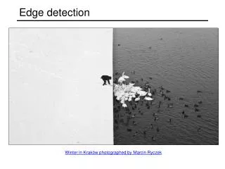
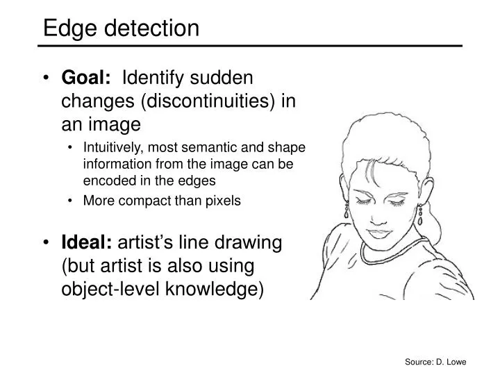
Edge detection. Goal: Identify sudden changes (discontinuities) in an image Intuitively, most semantic and shape information from the image can be encoded in the edges More compact than pixels Ideal: artist’s line drawing (but artist is also using object-level knowledge). Source: D. Lowe.

E N D
Edge detection • Goal: Identify sudden changes (discontinuities) in an image • Intuitively, most semantic and shape information from the image can be encoded in the edges • More compact than pixels • Ideal: artist’s line drawing (but artist is also using object-level knowledge) Source: D. Lowe
Origin of Edges • Edges are caused by a variety of factors surface normal discontinuity depth discontinuity surface color discontinuity illumination discontinuity Source: Steve Seitz
intensity function(along horizontal scanline) first derivative edges correspond toextrema of derivative Characterizing edges • An edge is a place of rapid change in the image intensity function image
Image gradient • The gradient of an image: • The gradient points in the direction of most rapid increase in intensity • The gradient direction is given by • how does this relate to the direction of the edge? • The edge strength is given by the gradient magnitude Source: Steve Seitz
Recall, for 2D function, f(x,y): This is linear and shift invariant, so must be the result of a convolution. We could approximate this as (which is obviously a convolution) Differentiation and convolution Source: D. Forsyth, D. Lowe
Finite difference filters • Other approximations of derivative filters exist: Source: K. Grauman
Finite differences: example • Which one is the gradient in the x-direction (resp. y-direction)?
Where is the edge? Effects of noise • Consider a single row or column of the image • Plotting intensity as a function of position gives a signal Source: S. Seitz
Effects of noise • Finite difference filters respond strongly to noise • Image noise results in pixels that look very different from their neighbors • Generally, the larger the noise the stronger the response • What is to be done? Source: D. Forsyth
Effects of noise • Finite difference filters respond strongly to noise • Image noise results in pixels that look very different from their neighbors • Generally, the larger the noise the stronger the response • What is to be done? • Smoothing the image should help, by forcing pixels different to their neighbors (=noise pixels?) to look more like neighbors Source: D. Forsyth
g f * g • To find edges, look for peaks in Solution: smooth first f Source: S. Seitz
f Derivative theorem of convolution • Differentiation is convolution, and convolution is associative: • This saves us one operation: Source: S. Seitz
Derivative of Gaussian filter • Is this filter separable? * [1 -1] =
Derivative of Gaussian filter • Which one finds horizontal/vertical edges? y-direction x-direction
Summary: Filter mask properties • Filters act as templates • Highest response for regions that “look the most like the filter” • Dot product as correlation • Smoothing masks • Values positive • Sum to 1 → constant regions are unchanged • Amount of smoothing proportional to mask size • Derivative masks • Opposite signs used to get high response in regions of high contrast • Sum to 0 → no response in constant regions • High absolute value at points of high contrast Source: K. Grauman
Tradeoff between smoothing and localization • Smoothed derivative removes noise, but blurs edge. Also finds edges at different “scales”. 1 pixel 3 pixels 7 pixels Source: D. Forsyth
Implementation issues • The gradient magnitude is large along a thick “trail” or “ridge,” so how do we identify the actual edge points? • How do we link the edge points to form curves? Source: D. Forsyth
Edge finding We wish to mark points along the curve where the magnitude is biggest. We can do this by looking for a maximum along a slice normal to the curve (non-maximum suppression). These points should form a curve. There are then two algorithmic issues: at which point is the maximum, and where is the next one? Source: D. Forsyth
Non-maximum suppression At q, we have a maximum if the value is larger than those at both p and at r. Interpolate to get these values. Source: D. Forsyth
Predicting the next edge point Assume the marked point is an edge point. Then we construct the tangent to the edge curve (which is normal to the gradient at that point) and use this to predict the next points (here either r or s). Source: D. Forsyth
Designing an edge detector • Criteria for an “optimal” edge detector: • Good detection: the optimal detector must minimize the probability of false positives (detecting spurious edges caused by noise), as well as that of false negatives (missing real edges) • Good localization: the edges detected must be as close as possible to the true edges • Single response: the detector must return one point only for each true edge point; that is, minimize the number of local maxima around the true edge Source: L. Fei-Fei
Canny edge detector • This is probably the most widely used edge detector in computer vision • Theoretical model: step-edges corrupted by additive Gaussian noise • Canny has shown that the first derivative of the Gaussian closely approximates the operator that optimizes the product of signal-to-noise ratio and localization J. Canny, A Computational Approach To Edge Detection, IEEE Trans. Pattern Analysis and Machine Intelligence, 8:679-714, 1986. Source: L. Fei-Fei
Canny edge detector • Filter image with derivative of Gaussian • Find magnitude and orientation of gradient • Non-maximum suppression: • Thin multi-pixel wide “ridges” down to single pixel width • Linking and thresholding (hysteresis): • Define two thresholds: low and high • Use the high threshold to start edge curves and the low threshold to continue them • MATLAB: edge(image, ‘canny’) Source: D. Lowe, L. Fei-Fei
The Canny edge detector • original image (Lena)
The Canny edge detector • norm of the gradient
The Canny edge detector • thresholding
The Canny edge detector • thinning • (non-maximum suppression)
high threshold (strong edges) low threshold (weak edges) hysteresis threshold Hysteresis thresholding original image Source: L. Fei-Fei
Effect of (Gaussian kernel spread/size) original Canny with Canny with • The choice of depends on desired behavior • large detects large scale edges • small detects fine features Source: S. Seitz
Edge detection is just the beginning… • Berkeley segmentation database:http://www.eecs.berkeley.edu/Research/Projects/CS/vision/grouping/segbench/ human segmentation image gradient magnitude