Download
1 / 44
440 likes | 444 Views
The Diffusion Region of Asymmetric Magnetic Reconnection. Michael Shay – Univ. of Delaware Bartol Research Institute. Collaborators. Paul Cassak Our Asymmetric reconnection publications (no guide field): General Scaling theory and resistive MHD:

E N D
The Diffusion Region of Asymmetric Magnetic Reconnection Michael Shay – Univ. of Delaware Bartol Research Institute
Collaborators • Paul Cassak • Our Asymmetric reconnection publications (no guide field): • General Scaling theory and resistive MHD: • Cassak and Shay, Physics of Plasmas, 14, 102114, 2007. • Hall MHD simulations • Cassak and Shay, GRL, (In press)
Semantics • Diffusion region • A non-MHD region where at least one species is not frozen-in • Not necessarily irreversible dissipation • Example: Hall region of regular collisionless reconnection.
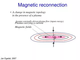
Y X Z Magnetic Reconnection Vin d CA Process breaking the frozen-in constraint determines the width of the dissipation region, d.
Magnetic Reconnection Simulation Jz and Magnetic Field Lines Y X
Reconnection drives convection in the Earth’sMagnetosphere. • d Kivelson et al., 1995
Reconnection in Solar Flares • X-class flare: t ~ 100 sec. • B ~ 100 G, n ~ 1010 cm-3 , L ~ 109 cm • tA ~ L/cA ~ 10 sec. F. Shu, 1992
Vin d cA D Y X Z Calculating Reconnection Rate • Reconnection rate Vin • Conservation of mass: Flow into and out of dissipation region: Vin ~ (d /D) cA • d determined by the process breaking the frozen-in constraint. => The spatial extent of the dissipation region is of key importance to determining the reconnection rate.
Y X Z Two Types of 2D Reconnection • d << D Vin << cA => Slow • d ~ D Vin ~ cA => Fast Out of Plane Current D Out of Plane Current D
Vi Ji Y Je X Z Kinetic Reconnection (cont.) • dissipation region in hybrid model ( Shay, et al., 1999) • Effect of Hall Physics • Ion dissipation region • Controls R. RateVin ~ (c/pi/Di) cA(c/pi/Di) ~ 1/10No system size Dependence! • Electron dissipation region • No impact on R. RateVine ~ (c/pe/De) cAe c/pi Di c/pe De
Whistler signature • Magnetic field from particle simulation (Pritchett, UCLA) • Self generated out-of-plane field is whistler signature • Confirmed with satellite and laboratory measurements.
Overview: Asymmetric Reconnection • What is Asymmetric Reconnection? • Diffusion region analysis • Resistive MHD Simulations • No guide field • Hall MHD Simulations • No guide field • Conclusions
Asymmetric Reconnection • Different B,n on either side of diffusion region. • Dayside magnetosphere • Solar reconnection? • Heliopause reconnection
Intense currents • MHD not valid • No frozen-in High nLow B • d Low nHigh B Kivelson et al., 1995
Observation • Asymmetric • Reconnecting B-field • Density • Temperature
Previous Work • Shock structure • Petschek slow shocks => Intermediate wave+expansion fan (Levy et al., 1964) • Further work • Petschek and Thorne, 1967; Sonnerup, 1974; Cowley, 1974; Semenov et al., 1983, MHD (Hoshino and Nishida, 1983; Scholer, 1989; Shi and Lee, 1990; Lin and Lee, 1993; La Belle-Hamer et al., 1995; Ku and Sibeck, 1997; Ugai, 2000; …), Kinetic - Hybrid: (Lin and Lee, 1993; Lin and Xie, 1997; Omidi et al, 1998; Krauss-Varban et al., 1999; Nakamura and Scholer, 2000; …),Particle: - Okuda, 1993. • Other relevant studies: Ding et al., 1992; Karimabadi et al., 1999; Siscoe et al., 2002; Swisdak et al., 2003; Linton, 2006; many dayside studies • Scaling studies undertaken only recently • Diamagneticd Stabilization (Swisdak et al., 2003) • Orientation of X-line, outflow speed (Swisdak and Drake, 2007) • MHD studies: (Borovsky and Hesse, 2007, Birn et al., 2008) • Global MHD (Borovosky et al., 2008) • PIC: (Pritchett, 2008), Tanaka, 2008; Huang et al., 2008 • PIC-Satellite comparisons (Mozer, Pritchett et al., 2008)
Conservation Laws • Write MHD in conservative form ( = mass density, v = flow velocity, B = magnetic field, P = pressure, E = electric field, • Integrate over closed surface. = total energy)
1 v1 B1 out 2 2L vout 2 B2 v2 More General Diffusion Region • Steady state diffusion relation • Integrate conservation relations Conservation of mass Conservation of momentum Conservation of Energy B/t = 0
1 v1 B1 out 2 2L vout 2 B2 v2 More General Diffusion Region • Steady state diffusion relation • Integrate conservation relations Conservation of mass Conservation of momentum Conservation of Energy B/t = 0
Asymmetric Scaling Relations • Solving gives • Need out Outflow speed Reconnection Rate
L A1 1 2 L A2 Outflow Density? • Assume reconnected flux tubes mix and conserve total volume. • Each flux tube contains same amount of flux: • B1A1 ~ B2A2
Weak field B1 Strong field B2 Weak field B1 X1 X X2 Strong field B2 Structure of the Dissipation Region • Since v1 B1 ~ v2 B2, the stronger magnetic field flows in slower • So it makes sense that the X-line is displaced toward the strong field side ofthe dissipation region.But this is incorrect! • The X-line is actually shifted toward the weak field side! • Why? While the flow coming in the strong field side is slower, the flux of energy is larger.
B1 v1 1 out X1 X2 2L vout B2 v2 2 Calculation of Location of X-line • Evaluate conservation of energy for volume from edge to X-line X Their ratio gives:
B2 v1 B1, 1 S1 S2 B2, 2 v2 Location of the Stagnation Point • Similar argument for mass flux • Stagnation point offset toward side with smaller B/. S
X-line and Stagnation Point are not colocated! • There is a flow across the X-line • Generic to asymmetric reconnection! • Previous magnetopause simulations (Siscoe, 2002; Dorelli et al., 2007, …) • Quantitative predictions of the location of X-line and stagnation point (Cassak and Shay, 2007) have been questioned (Birn et al., 2008)
Which plasma flows across the X-line? • Inflow Alfven speeds control flow across X-line Since cAsp > cAsh there is a flow of magnetosheath plasma in to magnetosphere. (Matches observations.)
Results are General • These relations giveE andvout in terms of upstream parameters. • No specificaion of diffusion mechanism or Hall term. • General applicability • Require diffusion (non-MHD) mechanism to determine absolute values: • Sets diffusion region widths and L • Determines actual reconnection rate
Resistive MHD • To find an absolute reconnection rate, we need to specify a dissipation mechanism. For asymmetric Sweet-Parker, • Uniform resistivity Sweet-Parker reconnection
Fluid Simulations • Double current sheet configuration • x = outflow y = out-of-plane z = inflow • B, T tanh functions • n balances B2
Resistive MHD Simulations • V normalized to cA, Length normalized to L0 • Size: 409.6 X 204.8, 4096 X 2048 grids • 0.05 • (Lundquist number = 8,192-40,960) • min = 1 initially • n1 = n2 • [B1,B2] = [1,1], [2,1], [3,1], [4,1], [5,1], [4,2]
Resistive MHD Simulations • [B1,B2] = [1,3] • [n1,n2] = [1,1] • x = outflow y = out-of-plane z = inflow
MHD Results Out-of-plane current density J Cut across X-linealong inflow S X Cut across X-linealong inflow Decoupling of X-line and stagnation point borne out in MHD simulations.
MHD Results • Color = out-of-plane currentWhite = magnetic field lines • Initial field asymmetry = 3,no density asymmetry • Signatures • Typical “bulge” into low-field region • Particles flow acrossX-line
Flux out Flux in Energy and Mass Flux Check • Determined geometry of diffusion region from simulations. • Non-trivial • Energy and Mass Flux balances in each sub-region
Verification of Scaling • Scaling laws for outflow speed vout and reconnection rate E in terms of geometry and upstream parameters tested • Very good agreement • Other studies find agreement: • Borovsky and Hesse, 2007 (anomalous resistivity MHD) • Birn et al., 2008 (Anomalous resistivity MHD) • Borovsky et al., 2008 (Global MHD) • Pritchett, 2008 (Kinetic PIC) vout E E
Hall MHD Simulations • Two dimensional Hall-MHD simulations • Anti-parallel magnetic fields • Three sets of runs • Asymmetric fields [B01,B02] = [1,1], [2,1], [3,1], [0.5,1], Symmetric density • Asymmetric density [n01,n02] = [1,1], [2,1], [3,1], [0.5,1], Symmetric field • Asymmetric density and field [B01(n01),B02(n02)] = [2(1),1(2)], [1(1),0.5(4)] • Asymmetric initial temperature to balance pressure • Box size = 204.8 x 102.4 c / pi • Grid scale = 0.05 c / pi • me = mi / 25 (density asymmetry not included in electron inertia term) • min = 4 initially
Hall MHD Simulations • [B1,B2] = [1,2] • [n1,n2] = [2,1] • x = outflow y = out-of-plane z = inflow
Hall-MHD Results • Electron and ion stagnation points different! Cuts across x-line along inflow Top - field lines (white) and out-of-plane magnetic field (color)Bottom - electron (black) and ion (white) flow lines and out-of-plane current (color) Initial field asymmetry = 3
Verification of Scaling • Generalized Sweet-Parker like scaling is satisfied for both electrons and ions. vout (electrons) vout (ions) E theory
The Big PictureMagnetospheric Applications? • Agreement of the scaling of E for Hall reconnection / L ~ 0.1 is independent of the asymmetry in B and • Are the results applicable to dayside magnetopause reconnection? • Yes (Borovsky) • In global MHD simulations, the reconnection rate at the nose of the magnetopause agreed with E based on local parameters rather than the solar wind electric field (Borovsky et al., 2008). • No (Dorelli) • The analysis is manifestly two-dimensional, whereas 3D effects (such as flows) are important at the magnetopause. • The orientation of the X-line between arbitrary fields not predicted. • Critical Question: • Can significant portions of dayside reconnection be characterized as quasi-2D? • Does a fluid element traversing the diffusion region see 3D effects?
Scaling of reconnection is a potential starting point for a quantitative understanding of solar wind-magnetospheric coupling Solar Wind-Magnetospheric Coupling Models • Newell et al., 2007 • Best model to date, but it uses ad hoc fitting to achieve performance • Borovsky (2008) usedour scaling result to derivea coupling function fromfirst principles • It performed as well as Newell’s
Conclusion • We have derived the scaling of the reconnection rate and outflow speed with upstream parameters during asymmetric reconnection [Cassak and Shay, Phys. Plasmas 14, 102114 (2007)] • Numerical simulations agree with the theory for collisional and collisionless (Hall) reconnection • Signatures of Asymmetric Reconnection • X-line and stagnation point not coincident for asymmetric B field • There is a bulk flow across the X-line • Potential applications to the dayside magnetosphere (Borovsky, 2008; Turner et al., in prep), though future work is needed
Future Directions • Much work to be done • Effect of guide field • Diamagnetic stabilization (Swisdak et al., 2003) • Orientation of X-line (Swisdak et al, 2007) • More realistic two-scale diffusion region • Requires Kinetic PIC • Pritchett, 2007 • Separatrix structures • Mozer et al., 2007 • Linking separatrix structures with diffusion region structure.