Download
1 / 17
170 likes | 273 Views
WEMBA 2000 Real Options 60. Call Option Delta. Call Price Curve: The Call Price as a function of the underlying asset price. Call value. Time to expiration decreases. As time to expiration decreases, the call price curve tends towards the payoff function (the payoff from

E N D
WEMBA 2000 Real Options 60 Call Option Delta Call Price Curve: The Call Price as a function of the underlying asset price Call value Time to expiration decreases As time to expiration decreases, the call price curve tends towards the payoff function (the payoff from the call at expiration). K S: Price of Underlying Asset The call "delta" is the slope of the call price curve: Delta () = c S Call price curve Call value Call Delta S: Price of Underlying Asset
WEMBA 2000 Real Options 61 Replicating the Rigby Option Payoff by delta-hedging Stock Price Tree 138.68 92.96 t = 1 year rf = 6.3% = 40% u = e t = 1.4918 d = 1/u = 0.6703 62.32 62.32 41.77 41.77 28 28 28 18.77 18.77 12.58 12.58 8.43 5.65 Call Option Tree 136.42 83.39 1.00 Price 48.65 0.98 44.78 27.20 0.91 22.45 0.95 14.84 0.8 10.83 0.76 3.6 5.32 0.58 1.80 0.36 0 0.93 0.24 Delta 0 0 0
WEMBA 2000 Real Options 62 Reserve $14.8 (Call option value) Sell delta * 1.2 barrels = $26.88 Date Price Delta T=0 28 0.8 T=1 41.77 0.91 T=2 62.32 0.98 T=3 92.96 1.00 T=4 138.68 1.00 Invest remainder: $12.08 at 6.3% Re-hedge: sell further (0.91 - 0.8) * 1.2 barrels 0.11*1.2*41.77 = $5.51 $12.84 at year end = $18.35 Invest at 6.3% + Re-hedge: sell further (0.98 - 0.91) * 1.2 barrels 0.07*1.2*62.32 = $5.23 = $24.75 Invest at 6.3% $19.51 at year end + = $28.53 Invest at 6.3% Re-hedge: sell further (1 - 0.98) * 1.2 barrels 0.02*1.2*92.96 = $2.23 $26.30 at year end + $30.33 at year end Buy back 1.2 barrels 1.2*138.68 = - $166.42 = - $136.09 + Exercise Option: (138.68 - 25)*1.2 = $136.41
WEMBA 2000 Real Options 63 Reserve $14.8 (Call option value) Sell delta * 1.2 barrels = $26.88 Date Price Delta T=0 28 0.8 T=1 41.77 0.91 T=2 28 0.76 T=3 18.77 0.36 T=4 28 1.00 Invest remainder: $12.08 at 6.3% Re-hedge: sell further (0.91 - 0.8) * 1.2 barrels 0.11*1.2*41.77 = $5.51 $12.84 at year end = $18.35 Invest at 6.3% + Re-hedge: buy back (0.76 - 0.91) * 1.2 barrels - 0.15*1.2*28 = - $5.04 = $14.47 Invest at 6.3% $19.51 at year end + = $6.37 Invest at 6.3% Re-hedge: buy back (0.36 - 0.76) * 1.2 barrels -0.4*1.2*18.77 = -$9.01 $15.38 at year end + Buy back remaining barrels - 0.36*1.2*28 = -$12.096 $6.77 at year end = -$5.326 + Exercise Option: (28 - 25)*1.2 = $3.6
WEMBA 2000 Real Options 64 Sources of Error Inevitable concerns when using the replicating portfolio (apply to financial options as well) How often to update the delta-hedge? Tradeoff between transactions costs and imperfect hedging Borrowing/lending rate: we cannot guarantee that our borrow/lend costs will remain unchanged Implied volatility: if we use the "wrong" implied vol, the delta will be wrong (e.g. set = 0.85 in first leg of Rigby hedge and re-evaluate the delta-hedging strategy) Short selling: we need to short-sell oil to hedge our exposure to a drop in oil prices. Further concerns in the case of real options: inputs in the Black-Scholes model Strike price: are we sure about the exact extraction costs throughout the project? (consider the example in the homework) Time to expiration: are we sure we have the right time frame? (suppose we are uncertain that the entire extraction can be completed in one year) Is the traded underlying asset a good proxy for the "real" underlying asset? Tracking risk...
WEMBA 2000 Real Options 65 Case Study: Natural Resources Abandonment Option Abbeytown Copper Refinery has two-year lease over a copper deposit. We have the following information: Deposit contains eight million pounds of copper Mining involves a one-year development phase, at a cost of $1.25 million immediately Extraction costs (outsourced) at $0.85 / pound at beginning of extraction phase (one year after development phase is initiated) Sale of copper would be at spot price of copper as of beginning of extraction phase Current spot price of copper is $0.95 / pound Copper prices are normally distributed with mean 7% and standard deviation 20% (p.a.) Abbeytown's required rate of return for this project is 10%, and the riskless rate is 5%
WEMBA 2000 Real Options 66 Case Study: Natural Resources Abandonment Option (2) Traditional NPV analysis: Expected NPV = -1.25 + 8(E[S1] - 0.85) 1.1 where E[S1] = Expected price of Copper in one year's time Current price of Copper, S0 = 0.95 Expected rate of return on copper, r = 7% Expected price of copper in one year, S1= 0.95e0.07= 1.0189 Hence E[NPV] = -1.25 + 8(1.0189 - 0.85)/1.1 = - 0.022 Reject Option Analysis S = 0.95 * 8 = 7.6 Call value = 1.3 K = 0.85 * 8 = 6.8 Option cost = 1.25 r = 5% O-A PV = 0.05 Accept T = 1 year = 20%
WEMBA 2000 Real Options 67 Case Study: Natural Resources Abandonment Option (3) Why does the option to abandon have value? Can choose to abandon the project if the price of copper is low after one year. Probability that we will abandon = 1 - Prob(exercise) = 1 - N(d2) = 1 - 0.76 = 0.24 The usual caveats…. How certain are we about the inputs? -- size of deposit ("real" option caveat) -- development costs and timing ("real" option caveat) -- extraction costs and timing ("real" option caveat) -- volatility of copper price over the next year (applies in any option pricing context) -- riskless borrow/lend rate (applies in any option pricing context)
WEMBA 2000 Real Options 68 Case Study: Prudence Properties Prudence Properties holds an option to sell a piece of commercial property that it currently owns, in six weeks time, for a price of $50 million. We have the following information: Ownership of the property is in the form of a REIT (Real Estate Investment Trust) hence we can observe the price of the property in the financial markets. Current price in the market is $50 million, and historic price volatility is 40% per year. The riskfree rate of interest is 10% per annum. Scenario 1: The option is European (can only be exercised at the end of the six week period).
WEMBA 2000 Real Options 69 Case Study: Prudence Properties (2) Scenario 1 cont.: The put option is European (can only be exercised at the end of the six week period). Take this on trust. The mathematical justification is ugly! Now we evaluate the option using a Binomial Tree model, as follows: S = 50 K = 50 rf = 10% T = 5/12 = 40% t = length (in yrs) of one "time-step" = 1/12 u = proportional change in S on an up-move = et = 1.224 d = proportional change in S on a down-move = 1/u = 0.8909 p = (ert - d)/(u - d) = 0.5076 89.07 0 79.35 0 70.70 0 70.70 0 62.99 0.63 62.99 0 56.12 0 56.12 1.30 56.12 2.11 50.00 4.32 50.00 3.67 50.00 2.66 44.55 5.45 44.55 6.66 44.55 6.17 39.69 9.86 39.69 9.90 35.36 14.64 35.36 13.81 Why is this result different from the Black-Scholes formula? 31.50 18.08 28.07 21.93
62.99 0.63 56.12 1.30 56.12 2.11 50.00 4.32 50.00 3.67 50.00 2.66 44.55 5.45 44.55 6.66 44.55 6.17 39.69 9.86 39.69 9.90 35.36 14.64 35.36 13.81 31.50 18.08 28.07 21.93 WEMBA 2000 Real Options 70 Case Study: Prudence Properties (3) Scenario 2: The put option is American (can be exercised at any time during the six week period). Compare the original tree… … with the value of immediate exercise at each node 62.99 0.63 56.12 1.30 56.12 2.16 50.00 4.49 50.00 3.77 50.00 2.66 44.55 5.45 44.55 6.96 44.55 6.38 39.69 10.36 39.69 10.31 35.36 14.64 35.36 14.64 Binomial method for Amer put with 100 steps: put price = 4.30 31.50 18.50 28.07 21.93
WEMBA 2000 Real Options 71 Case Study: Prudence Properties (4) Scenario 3: The put option is European, and ownership of the property yields rental income of $2.06 MM in 3.5 months time. PV of rental income = 2.06e0.2917*0.1 = 2.00 How do we treat the lease payment prior to option expiration date: (a) add it up-front to the value of the option? (b) add it to the present value of the property? (c) subtract it from the strike price of the option? Add PV(2.6) upfront Total option value: 4.08 + 2.06 = $6.14 Add PV(2.06) to value of property Total option value: $3.36 Subtract PV(2.06) from strike Total option value: $3.20
62.99 56.12 56.12 50.00 50.00 50.00 44.55 44.55 44.55 39.69 39.69 35.36 35.36 31.50 28.07 WEMBA 2000 Real Options 72 Case Study: Prudence Properties (4) Scenario 4: The put option is American, and ownership of the property yields rental income of $2.06 MM in 3.5 months time. The market price of the property today is $52. Step 1: Construct a tree for S*, the property value without the rental income: S* = 50 (this is the same as the original tree in Scenario 1) Step 2: Adjust the tree by the present value of the dividend at each node 65.02 58.17 58.14 52.00 52.03 46.60 46.57 50.00 41.72 44.55 37.41 39.69 35.36 31.50 28.07
65.02 0.63 58.17 1.30 58.14 2.15 52.00 4.43 52.03 3.76 50.00 2.66 46.60 6.37 46.57 6.85 44.55 5.45 41.72 10.15 39.69 10.31 37.41 14.22 35.36 14.64 31.50 18.50 28.07 21.93 WEMBA 2000 Real Options 73 Case Study: Prudence Properties (5) Scenario 4 cont.: The put option is American, and ownership of the property yields rental income of $2.06 MM in 3.5 months time. The market price of the property today is $52. Price the American put by checking whether early exercise is optimal at each point… … and compare with the European put with the rental income (Scenario 2) 65.51 0.43 58.36 0.88 58.36 1.62 52.00 3.56 52.00 2.87 52.00 1.79 46.33 3.67 46.33 5.62 46.33 4.96 41.28 8.55 41.28 8.31 36.78 13.22 36.78 12.40 32.77 16.82 29.19 20.81
WEMBA 2000 Real Options 74 Case Study: Prudence Properties -- Summary European-styleAmerican-style Rental Income Rental Income $0 $2.06 $0 $2.06 4.08 3.36 n/a n/a 4.32 3.56 4.49 4.43 Black-Scholes Binomial tree 5 Steps
WEMBA 2000 Real Options 75 Estimating Historical Volatility
WEMBA 2000 Real Options 76 Estimating Historical Volatility Define: n+1 = # of observations Si = asset price at end of ith interval (i = 0,1,2,…, n) T = length of time interval (years) Now let ui = ln (Si / Si-1 ) Then ui is the continuously compounded return on the asset in the ith interval The standard deviation s of the returns vi is given by: s = [1/(n-1) n ( ui - û )2] where û is the mean of the ui ‘s.