Download
1 / 52
520 likes | 671 Views
Non-linear effects Yannis PAPAPHILIPPOU Accelerator and Beam Physics group Beams Department CERN. Joint University Accelerator School Archamps, FRANCE 22-24 January 2014. Bibliography. Books on non-linear dynamical systems

E N D
Non-linear effectsYannis PAPAPHILIPPOUAccelerator and Beam Physics groupBeams DepartmentCERN Joint University Accelerator School Archamps, FRANCE 22-24 January 2014
Bibliography • Books on non-linear dynamical systems • M. Tabor, Chaos and Integrability in Nonlinear Dynamics, An Introduction, Willey, 1989. • A.J Lichtenberg and M.A. Lieberman, Regular and Chaotic Dynamics, 2nd edition, Springer 1992. • Books on beam dynamics • E. Forest, Beam Dynamics - A New Attitude and Framework, Harwood Academic Publishers, 1998. • H. Wiedemann, Particle accelerator physics, 3rd edition, Springer 2007. • Lectures on non-linear beam dynamics • A. Chao, Advanced topics in Accelerator Physics, USPAS, 2000. • A. Wolski, Lectures on Non-linear dynamics in accelerators, Cockroft Institute 2008. • W. Herr, Lectures on Mathematical and Numerical Methods for Non-linear Beam Dynamics in Rings, CAS 2013. • L. Nadolski, Lectures on Non-linear beam dynamics, Master NPAC, LAL, Orsay 2013.
Contents of the 1st lecture • Accelerator performance parameters and non-linear effects • Linear and non-linear oscillators • Integral and frequency of motion • The pendulum • Damped harmonic oscillator • Phase space dynamics • Fixed point analysis • Non-autonomous systems • Driven (damped) harmonic oscillator, resonance conditions • Linear equations with periodic coefficients – Hill’s equations • Floquet solutions and normalized coordinates • Perturbation theory • Non-linear oscillator • Perturbation by periodic function – single dipole perturbation • Application to single multipole – resonance conditions • Examples: single quadrupole, sextupole, octupole perturbation • General multi-pole perturbation– example: linear coupling • Resonance conditions and working point choice • Summary • Appendix I: Multipole expansion
Contents of the 1st lecture • Accelerator performance parameters and non-linear effects • Linear and non-linear oscillators • Integral and frequency of motion • The pendulum • Damped harmonic oscillator • Phase space dynamics • Fixed point analysis • Non-autonomous systems • Driven (damped) harmonic oscillator, resonance conditions • Linear equations with periodic coefficients – Hill’s equations • Floquet solutions and normalized coordinates • Perturbation theory • Non-linear oscillator • Perturbation by periodic function – single dipole perturbation • Application to single multipole – resonance conditions • Examples: single quadrupole, sextupole, octupole perturbation • General multi-pole perturbation– example: linear coupling • Resonance conditions and working point choice • Summary • Appendix I: Multipole expansion
Accelerator performance parameters • Colliders • Luminosity (i.e. rate of particle production) • Νbbunch population • kb number of bunches • γ relativistic reduced energy • εn normalized emittance • β* “betatron” amplitude function at collision point • High intensity accelerators • Average beam power • mean current intensity • Εenergy • fN repetition rate • Νnumber of particles/pulse • Synchrotron light sources (low emittance rings) • Brightness (photon density in phase space) • Νpnumber of photons • εx,,ytransverse emittances I Non-linear effects limit performance of particle accelerators but impact also design cost
Non-linear effects in colliders Limitations affecting (integrated) luminosity Particle losses causing Reduced lifetime Radio-activation (super-conducting magnet quench) Reduced machine availability Emittance blow-up Reduced number of bunches (either due to electron cloud or long-range beam-beam) Increased crossing angle Reduced intensity Cost issues Number of magnet correctors and families (power convertors) Magnetic field and alignment tolerances • At injection • Non-linear magnets (sextupoles, octupoles) • Magnet imperfections and misalignments • Power supply ripple • Ground motion (for e+/e-) • Electron (Ion) cloud • At collision • Insertion Quadrupoles • Magnets in experimental areas (solenoids, dipoles) • Beam-beam effect (head on and long range)
Non-linear effects in high-intensity accelerators Limitations affecting beam power Particle losses causing Reduced intensity Radio-activation (hands-on maintenance) Reduced machine availability Emittance blow-up which can lead to particle loss Cost issues Number of magnet correctors and families (power convertors) Magnetic field and alignment tolerances Design of the collimation system • Non-linear magnets (sextupoles, octupoles) • Magnet imperfections and misalignments • Injection chicane • Magnet fringe fields • Space-charge effect
Non-linear effects in low emittance rings Limitations affecting beam brightness Reduced injection efficiency Particle losses causing Reduced lifetime Reduced machine availability Emittance blow-up which can lead to particle loss Cost issues Number of magnet correctors and families (power convertors) Magnetic field and alignment tolerances • Chromaticity sextupoles • Magnet imperfections and misalignments • Insertion devices (wigglers, undulators) • Injection elements • Ground motion • Magnet fringe fields • Space-charge effect (in the vertical plane for damping rings) • Electron cloud (Ion) effects
Contents of the 1st lecture • Accelerator performance parameters and non-linear effects • Linear and non-linear oscillators • Integral and frequency of motion • The pendulum • Damped harmonic oscillator • Phase space dynamics • Fixed point analysis • Non-autonomous systems • Driven (damped) harmonic oscillator, resonance conditions • Linear equations with periodic coefficients – Hill’s equations • Floquet solutions and normalized coordinates • Perturbation theory • Non-linear oscillator • Perturbation by periodic function – single dipole perturbation • Application to single multipole – resonance conditions • Examples: single quadrupole, sextupole, octupole perturbation • General multi-pole perturbation– example: linear coupling • Resonance conditions and working point choice • Summary • Appendix I: Multipole expansion
Reminder: Harmonic oscillator • Described by the differential equation: • The solution obtained by the substitution and the solutions of the characteristic polynomial are which yields the general solution • The amplitude and phase depend on the initial conditions • Note that a negative sign in the differential equation provides a solution described by an hyperbolic sine function • Note also that for no restoring force , the motion is unbounded
Integral of motion • Rewrite the differential equation of the harmonic oscillator as a pair of coupled 1st order equations which can be combined to provide or with an integral of motion identified as the mechanical energy of the system • Solving the previous equation for , the system can be reduced to a first order equation
Integration by quadrature • The last equation can be be solved as an explicit integral or “quadrature” , yielding or the well-known solution • Note: Although the previous route may seem complicated, it becomes more natural when non-linear terms appear, where a substitution of the type is not applicable • The ability to integrate a differential equation is not just a nice mathematical feature, but deeply characterizes the dynamical behavior of the system described by the equation
Frequency of motion The period of the harmonic oscillator is calculated through the previous integral after integration between two extrema (when the velocity vanishes), i.e. : The frequency (or the period) of linear systems is independent of the integral of motion (energy) Note that this is not true for non-linear systems, e.g. for an oscillator with a non-linear restoring force The integral of motion is and the integration yields This means that the period (frequency) depends on the integral of motion (energy) i.e. the maximum “amplitude”
The pendulum An important non-linear equation which can be integrated is the one of the pendulum, for a string of length L and gravitational constant g For small displacements it reduces to an harmonic oscillator with frequency The integral of motion (scaled energy) is and the quadrature is written as assuming that for
Solution for the pendulum Using the substitutions with , the integral is and can be solved using Jacobi elliptic functions: For recovering the period, the integration is performed between the two extrema, i.e. and , corresponding to and , for which i.e. the complete elliptic integral multiplied by four times the period of the harmonic oscillator
Damped harmonic oscillator I • Damped harmonic oscillator: • is the ratio between the stored and lost energy per cycle with the damping ratio • is the eigen-frequency of the harmonic oscillator • General solution can be found by the same ansatz leading to an auxiliary 2nd order equation with solutions
Damped harmonic oscillator II • Three cases can be distinguished • Overdamping( real, i.e. or ): The system exponentially decays to equilibrium (slower for larger damping ratio values) • Criticaldamping(ζ = 1): The system returns to equilibrium as quickly as possible without oscillating. • Underdamping( complex, i.e. or ): The system oscillates with the amplitude gradually decreasing to zero, with a slightly different frequency than the harmonic one: • Note that there is no integral of motion, in that case, as the energy is not conserved (dissipative system)
Contents of the 1st lecture • Accelerator performance parameters and non-linear effects • Linear and non-linear oscillators • Integral and frequency of motion • The pendulum • Damped harmonic oscillator • Phase space dynamics • Fixed point analysis • Non-autonomous systems • Driven (damped) harmonic oscillator, resonance conditions • Linear equations with periodic coefficients – Hill’s equations • Floquet solutions and normalized coordinates • Perturbation theory • Non-linear oscillator • Perturbation by periodic function – single dipole perturbation • Application to single multipole – resonance conditions • Examples: single quadrupole, sextupole, octupole perturbation • General multi-pole perturbation– example: linear coupling • Resonance conditions and working point choice • Summary • Appendix I: Multipole expansion
Phase space dynamics Valuable description when examining trajectories in phase space Existence of integral of motion imposes geometrical constraints on phase flow For the harmonic oscillator (left), phase space curves are ellipses around the equilibrium point parameterized by the integral of motion (energy) By simply changing the sign of the potential in the harmonic oscillator (right), the phase trajectories become hyperbolas, symmetric around the equilibrium point where two straight lines cross, moving towards and away from it For the damped harmonic oscillator (above), the phase space trajectories are spiraling towards equilibrium with a rate depending on the damping coefficient
Non-linear oscillators • Conservative non-linear oscillators have quadrature with potential being a general (polynomial) function of positions • The equations of motion are • Equilibrium points are associated with extrema of the potential • Considering three non-linear oscillators • Quartic potential (left): two minima and one maximum • Cubic potential (center): one minimum and one maximum • Pendulum (right): periodic minima and maxima
Fixed point analysis Consider a general second order system Equilibrium or “fixed” points are determinant for topology of trajectories at their vicinity The linearized equations of motion at their vicinity are Fixed point nature is revealed by eigenvalues of , i.e. solutions of the characteristic polynomial Jacobian matrix
Fixed point for conservative systems • For conservative systems of two dimensions the second order characteristic polynomial has too solutions: • Two complex eigenvalues with opposite sign, corresponding to elliptic fixed points. Phase space flow is described by ellipses, with particles evolving clockwise or anti-clockwise • Two real eigenvalues with opposite sign, corresponding to hyperbolic (or saddle) fixed points. Flow described by two lines (or manifolds), incoming (stable) and outcoming (unstable) hyperbolic elliptic
Pendulum fixed point analysis • The “fixed” points for a pendulum can be found at • The Jacobian matrix is • The eigenvalues are • Two cases can be distinguished: • , for which corresponding to elliptic fixed points • , for which corresponding to hyperbolic fixed points • The separatrix are the stable and unstable manifolds passing through the hyperbolic points, separating bounded librationsand unbounded rotations elliptic hyperbolic
Contents of the 1st lecture • Accelerator performance parameters and non-linear effects • Linear and non-linear oscillators • Integral and frequency of motion • The pendulum • Damped harmonic oscillator • Phase space dynamics • Fixed point analysis • Non-autonomous systems • Driven (damped) harmonic oscillator, resonance conditions • Linear equations with periodic coefficients – Hill’s equations • Floquet solutions and normalized coordinates • Perturbation theory • Non-linear oscillator • Perturbation by periodic function – single dipole perturbation • Application to single multipole – resonance conditions • Examples: single quadrupole, sextupole, octupole perturbation • General multi-pole perturbation– example: linear coupling • Resonance conditions and working point choice • Summary • Appendix I: Multipole expansion
Non-autonomous systems Consider a linear system with explicit dependence in time Time now is not an independent variable but can be considered as an extra dimension leading to a completely new type of behavior Consider two independent solutions of the homogeneous equation and The general solution is a sum of the homogeneous solutions and a particular solution, , where the coefficients are computed as with the Wronskian of the system
Driven harmonic oscillator Consider periodic force pumping energy into the system General solution is a combination of the homogeneous and a particular solution found as Obviously a resonance condition appears when driving frequency hits the oscillator eigen-frequency. In the limit of the solution becomes The 2nd secular term implies unbounded growth of amplitude at resonance
Damped oscillator with periodic driving Consider periodic force pumping energy into the system The solution of the homogeneous system is The particular solution is The homogeneous solution vanishes for , leaving only the particular one, for which there is an amplitude maximum for but no divergence In that case the energy pumped into the system compensate the friction, a steady state representing a limit cycle
Phase space for non-autonomous systems Plotting the evolution of the driven oscillator in provides trajectories that intersect each other (top) The phase space has time as an extra 3rd dimension By rescaling the time to become and considering every integer interval of the new time variable, the phase space looks like the one of the harmonic oscillator (middle) This is the simplest version of a (Poincaré) surface of section, which is useful for studying geometrically phase space of multi-dimensional systems The fixed point in the surface of section is now a periodic orbit (bottom) defined by In that case, one can show the existence of two integrals of motion, but when a non-linearity is introduced, the system becomes non-integrable
Contents of the 1st lecture • Accelerator performance parameters and non-linear effects • Linear and non-linear oscillators • Integral and frequency of motion • The pendulum • Damped harmonic oscillator • Phase space dynamics • Fixed point analysis • Non-autonomous systems • Driven (damped) harmonic oscillator, resonance conditions • Linear equations with periodic coefficients – Hill’s equations • Floquet solutions and normalized coordinates • Perturbation theory • Non-linear oscillator • Perturbation by periodic function – single dipole perturbation • Application to single multipole – resonance conditions • Examples: single quadrupole, sextupole, octupole perturbation • General multi-pole perturbation– example: linear coupling • Resonance conditions and working point choice • Summary • Appendix I: Multipole expansion
Linear equation with periodic coefficients George Hill A very important class of equations especially for beam dynamics (but also solid state physics) are linear equations with periodic coefficients with a periodic function of time These are called Hill’s equations and can be thought as equations of harmonic oscillator with time dependent (periodic) frequency There are two solutions that can be written as with periodic but also with a constant which implies that is periodic The solutions are derived based on Floquet theory
Amplitude, phase and invariant Differentiating the solutions twice and substituting to Hill’s equation, the following two equations are obtained The 2nd one can be integrated to give , i.e. the relation between the “phase” and the amplitude Substituting this to the 1st equation, the amplitude equation is derived (or the beta function in accelerator jargon) By evaluating the quadratic sum of the solution and its derivative an invariant can be constructed, with the form
Normalized coordinates • Recall the Floquet solutions for betatron motion • Introduce new variables • In matrix form • Hill’s equation becomes • System becomes harmonic oscillator with frequency or • Floquet transformation transforms phase space in circles
Perturbation of Hill’s equations • Hill’s equations in normalized coordinates with harmonic perturbation, using and where the F is the Lorentz force from perturbing fields • Linear magnet imperfections: deviation from the design dipole and quadrupole fields due to powering and alignment errors • Time varying fields: feedback systems (damper) and wake fields due to collective effects (wall currents) • Non-linear magnets: sextupole magnets for chromaticity correction and octupole magnets for Landau damping • Beam-beam interactions: strongly non-linear field • Space charge effects: very important for high intensity beams • non-linear magnetic field imperfections: particularly difficult to control for super conducting magnets where the field quality is entirely determined by the coil winding accuracy
Contents of the 1st lecture • Accelerator performance parameters and non-linear effects • Linear and non-linear oscillators • Integral and frequency of motion • The pendulum • Damped harmonic oscillator • Phase space dynamics • Fixed point analysis • Non-autonomous systems • Driven (damped) harmonic oscillator, resonance conditions • Linear equations with periodic coefficients – Hill’s equations • Floquet solutions and normalized coordinates • Perturbation theory • Non-linear oscillator • Perturbation by periodic function – single dipole perturbation • Application to single multipole – resonance conditions • Examples: single quadrupole, sextupole, octupole perturbation • General multi-pole perturbation– example: linear coupling • Resonance conditions and working point choice • Summary • Appendix I: Multipole expansion
Perturbation theory Completely integrable systems are exceptional For understanding dynamics of general non-linear systems composed of a part whose solution is known and a part parameterized by a small constant , perturbation theory is employed The general idea is to expand the solution in a power series and compute recursively the corrections hoping that a few terms will be sufficient to find an accurate representation of the general solution This may not be true for all times, i.e. facing series convergence problems In addition, any series expansion breaks in the vicinity of a resonance
Perturbation of non-linear oscillator • Consider a non-linear harmonic oscillator, • This is just the pendulum expanded to 3rd order in • Note that is a dimensionless measure of smallness, which may represent a scaling factor of (e.g. without loss of generality) • Expanding and separating the equations with equal power in : • Order 0: • Order 1: • The 2nd equation has a particular solution with two terms. A well behaved one and the first part of which grows linearly with time (secular term) • But this cannot be true, the pendulum does not present such behavior. What did it go wrong?
Perturbation of non-linear oscillator It was already shown that the pendulum has an amplitude dependent frequency, so the frequency has to be developed as well (Poincaré-Linsteadmethod): Assume that the solution is a periodic function of which becomes the new independent variable. The equation at zero order gives the solution and at leading perturbation order becomes The last term has to be zero, if not it gives secular terms, thus which reveals the decrease of the frequency with the oscillation amplitude Finally, the solution is the leading order correction due to the non-linear term
Perturbation by periodic function In beam dynamics, perturbing fields are periodic functions The problem to solve is a generalization of the driven harmonic oscillator, with a general periodic function , with frequency The right side can be Fourier analyzed: The homogeneous solution is The particular solution can be found by considering that has the same form as : By substituting we find the following relation for the Fourier coefficients of the particular solution There is a resonance condition for infinite number of frequencies satisfying
Perturbation by single dipole Hill’s equations in normalized coordinates with single dipole perturbation: The dipole perturbation is periodic, so it can be expanded in a Fourier series Note, as before that a periodic kick introduces infinite number of integer driving frequencies The resonance condition occurs when i.e. integer tunes should be avoided (remember orbit distortion due to single dipole kick)
Perturbation by single multi-pole For a generalized multi-pole perturbation, Hill’s equation is: As before, the multipole coefficient can be expanded in Fourier series Following the perturbation steps, the zero-order solution is given by the homogeneous equation Then the position can be expressed as with The first order solution is written as
Resonances for single multi-pole Following the discussion on the periodic perturbation, the solution can be found by setting the leading order solution to be periodic with the same frequency as the right hand side Equating terms of equal exponential powers, the Fourier amplitudes are found to satisfy the relationship This provides the resonance condition or which means that there are resonant frequencies for and “infinite” number of rationals
Tune-shift for single multi-pole Note that for even multi-poles and or , there is a Fourier coefficient , which is independent of and represents the average value of the periodic perturbation The perturbing term in the r.h.s. is which can be obtained for (it is indeed an integer only for even multi-poles) Following the approach of the perturbed non-linear harmonic oscillator, this term will be secular unless a perturbation in the frequency is considered, thereby resulting to a tune-shift equal to with This tune-shift is amplitude dependent for
Example: single quadrupole perturbation Consider single quadrupole kick in one normalized plane: The quadrupole perturbation can be expanded in a Fourier series Following the perturbation approach, the 1st order equation becomes with For , the resonance conditions are i.e. integer and half-integer tunes should be avoided For , the condition corresponds to a non-vanishing average value , which can be absorbed in the left-hand side providing a tune-shift: or
Single Sextupole Perturbation Consider a localized sextupole perturbation in the horizontal plane After replacing the perturbation by its Fourier transform and inserting the unperturbed solution to the right hand side with Resonance conditions: Note that there is not a tune-spread associated. This is only true for small perturbations (first order perturbation treatment) Although perturbation treatment can provide approximations for evolution of motion, there is no exact solution 3rd integer integer
General multi-pole perturbation Equations of motion including any multi-pole error term, in both planes Expanding perturbation coefficient in Fourier series and inserting the solution of the unperturbed system on the rhs gives the following series: The equation of motion becomes In principle, same perturbation steps can be followed for getting an approximate solution in both planes
Example: Linear Coupling For a localized skew quadrupole we have Expanding perturbation coefficient in Fourier series and inserting the solution of the unperturbed system gives the following equation: with The coupling resonance are found for Linear sum resonance Linear difference resonance
General resonance conditions The general resonance conditions is or , with order The same condition can be obtained in the vertical plane For all the polynomial field terms of a -pole, the main excited resonances satisfy the condition but there are also sub-resonances for which For normal (erect) multi-poles, the main resonances are whereas for skew multi-poles If perturbation is large, all resonances can be potentially excited The resonance conditions form lines in the frequency space and fill it up as the order grows (the rational numbers form a dense set inside the real numbers)
Systematic and random resonances If lattice is made out of identical cells, and the perturbation follows the same periodicity, resulting in a reduction of the resonance conditions to the ones satisfying These are called systematic resonances Practically, any (linear) lattice perturbation breaks super-periodicity and any random resonance can be excited Careful choice of the working point is necessary
Contents of the 1st lecture • Accelerator performance parameters and non-linear effects • Linear and non-linear oscillators • Integral and frequency of motion • The pendulum • Damped harmonic oscillator • Phase space dynamics • Fixed point analysis • Non-autonomous systems • Driven (damped) harmonic oscillator, resonance conditions • Linear equations with periodic coefficients – Hill’s equations • Floquet solutions and normalized coordinates • Perturbation theory • Non-linear oscillator • Perturbation by periodic function – single dipole perturbation • Application to single multipole – resonance conditions • Examples: single quadrupole, sextupole, octupole perturbation • General multi-pole perturbation– example: linear coupling • Resonance conditions and working point choice • Summary • Appendix I: Multipole expansion
Summary • Accelerator performance depends heavily on the understanding and control of non-linear effects • The ability to integrate differential equations has a deep impact to the dynamics of the system • Phase space is the natural space to study this dynamics • Perturbation theory helps integrate iteratively differential equations and reveals appearance of resonances • Periodic perturbations drive infinite number of resonances • There is an amplitude dependent tune-shift at 1st order for even multi-poles • Periodicity of the lattice very important for reducing number of lines excited at first order