Download
1 / 24
240 likes | 363 Views
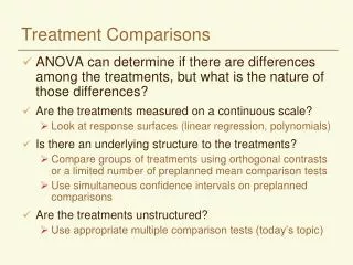
Treatment comparisons. ANOVA can determine if there are differences among the treatments, but what is the nature of those differences? Are the treatments measured on a continuous scale? Look at response surfaces (linear regression, polynomials)

E N D
Treatment comparisons • ANOVA can determine if there are differences among the treatments, but what is the nature of those differences? • Are the treatments measured on a continuous scale? • Look at response surfaces (linear regression, polynomials) • Is there an underlying structure to the treatments? • Compare groups of treatments using orthogonal contrasts or a limited number of preplanned mean comparison tests • Are the treatments unstructured? • Use appropriate mean comparison tests
Comparison of Means • Pairwise Comparisons • Least Significant Difference (LSD) • Simultaneous Confidence Intervals • Dunnett Test (making all comparisons to a control) • Bonferroni Inequality • Other Multiple Comparisons - “Data Snooping” • Fisher’s Protected LSD (FPLSD) • Student-Newman-Keuls test (SNK) • Tukey’s honestly significant difference (HSD) • Waller and Duncan’s Bayes LSD (BLSD) • False Discovery Rate Procedure • Often misused - intended to be used only for data from experiments with unstructured treatments
Multiple Comparison Tests • Fixed Range Tests – a constant value is used for all comparisons • Application • Hypothesis Tests • Confidence Intervals • Multiple Range Tests – values used for comparison vary across a range of means • Application • Hypothesis Tests
Variety Trials • In a breeding program, you need to examine large numbers of selections and then narrow to the best • In the early stages, based on single plants or single rows of related plants. Seed and space are limited, so difficult to have replication • When numbers have been reduced and there is sufficient seed, you can conduct replicated yield trials and you want to be able to “pick the winner”
= LSD 2 MSE / r t a Least Significant Difference • Calculating a t for testing the difference between two means • any difference for which the t > t would be declared significant • Further, is the smallest difference for which significance would be declared • therefore • or with equal replication, where r is number of observations forming the mean
Do’s and Don’ts of using LSD • LSD is a valid test when • making comparisons planned in advance of seeing the data (this includes the comparison of each treatment with the control) • Comparing adjacent ranked means • The LSD should not (unless F for treatments is significant) be used for • making all possible pairwise comparisons • making more comparisons than df for treatments
Pick the Winner • A plant breeder wanted to measure resistance to stem rust for six wheat varieties • planted 5 seeds of each variety in each of four pots • placed the 24 pots randomly on a greenhouse bench • inoculated with stem rust • measured seed yield per pot at maturity
Ranked Mean Yields (g/pot) Mean Yield Difference Variety Rank YiYi-1 - Yi F 1 95.3 D 2 94.0 1.3 E 3 75.0 19.0 B 4 69.0 6.0 A 5 50.3 18.7 C 6 24.0 26.3
= = = LSD 2 MSE / r 2.101 ( 2 * 120 ) / 4 16.27 t a = = = LSD 2 MSE / r 2.878 ( 2 * 120 ) / 4 22.29 t a ANOVA • Compute LSD at 5% and 1% Source df MS F Variety 5 2,976.44 24.80 Error 18 120.00
Back to the data... LSD=0.05 = 16.27 LSD=0.01 = 22.29 Mean Yield Difference Variety Rank YiYi-1 - Yi F 1 95.3 D 2 94.0 1.3 E 3 75.0 19.0* B 4 69.0 6.0 A 5 50.3 18.7* C 6 24.0 26.3**
Pairwise Comparisons • If you have 10 varieties and want to look at all possible pairwise comparisons • that would be t(t-1)/2 or 10(9)/2 = 45 • that’s a few more than t-1 df = 9 • LSD would only allow 9 comparisons
Type I vs Type II Errors • Type I error - saying something is different when it is really the same (Paranoia) • the rate at which this type of error is made is the significance level • Type II error - saying something is the same when it is really different (Sloth) • the probability of committing this type of error is designated b • the probability that a comparison procedure will pick up a real difference is called the power of the test and is equal to 1-b • Type I and Type II error rates are inversely related to each other • For a given Type I error rate, the rate of Type II error depends on • sample size • variance • true differences among means
Nobody likes to be wrong... • Protection against Type I is choosing a significance level • Protection against Type II is a little harder because • it depends on the true magnitude of the difference which is unknown • choose a test with sufficiently high power • Reasons for not using LSD for more than t-1 comparisons • the chance for a Type I error increases dramatically as the number of treatments increases • for example, with only 20 means - you could make a type I error 95% of the time (in 95/100 experiments)
Comparisonwise vs Experimentwise Error • Comparisonwise error rate ( = C) • measures the proportion of all differences that are expected to be declared real when they are not • Experimentwise error rate (E) • the risk of making at least one Type I error among the set (family) of comparisons in the experiment • measures the proportion of experiments in which one or more differences are falsely declared to be significant • the probability of being wrong increases as the number of means being compared increases
Comparisonwise vs Experimentwise Error • Experimentwise error rate (E) Probability of no Type I errors = (1-C)x where x = number of pairwise comparisons Max x = t(t-1)/2 , where t=number of treatments Probability of at least one Type I error E = 1- (1-C)x • Comparisonwise error rate C = 1- (1-E)1/x if t = 10, Max x = 45, E = 90%
LSD = tα 2MSE / r Fisher’s protected LSD (FPLSD) • Uses comparisonwise error rate • Computed just like LSD but you don’t use it unless the F for treatments tests significant • So in our example data, any difference between means that is greater than 16.27 is declared to be significant
BLSD = t 2MSE/r Waller-Duncan Bayes LSD (BLSD) • Do ANOVA and compute F (MST/MSE) with q and f df (corresponds to table nomenclature) • Choose error weight ratio, k • k=100 corresponds to 5% significance level • k=500 for a 1% test • Obtain tb from table (A7 in Petersen) • depends on k, F, q (treatment df) and f (error df) • Compute • Any difference greater than BLSD is significant • Does not provide complete control of experimentwise Type I error • Reduces Type II error
Duncan’s New Multiple-Range Test • Alpha varies depending on the number of means involved in the test Alpha 0.05 Error Degrees of Freedom 6 Error Mean Square 113.0833 Number of Means 2 3 4 5 6 Critical Range 26.02 26.97 27.44 27.67 27.78 Means with the same letter are not significantly different. Duncan Grouping Mean N variety A 95.30 2 6 A A 94.00 2 4 A B A 75.00 2 5 B A B A 69.00 2 2 B B 50.30 2 1 C 22.50 2 3
wherej=1,2,..., t-1, k=2,3,...,t = SNK MSE / r Q a,k, j Student-Newman-Keuls Test (SNK) • Rank the means from high to low • Compute t-1 significant differences, SNKj , using the HSD • Compare the highest and lowest • if less than SNK, no differences are significant • if greater than SNK, compare next highest mean with next lowest using next SNK • Uses experimentwise for the extremes and comparisonwise for adjacent
Using SNK with example data: k 2 3 4 5 6 Q 2.97 3.61 4.00 4.28 4.49 SNK 16.27 19.77 21.91 23.44 24.59 Mean Yield Variety Rank Yi F 1 95.3 D 2 94.0 E 3 75.0 B 4 69.0 A 5 50.3 C 6 24.0 5 4 3 2 1 =15 comparisons 18 df for error se= = SQRT(120/4) = 5.477 SNK=Q*se
HSD = Q MSE / r Tukey’s honestly significant difference (HSD) • From a table of studentized range values, select a value of Qa which depends on k (the number of means) and v (error df) (Appendix Table VII in Kuehl) • Compute HSD as • For any pair of means, if the difference is greater than HSD, it is significant • Uses an experimentwise error rate • Dunnett’s test is a special case where all treatments are compared to a control
Bonferroni Inequality E x * C where x = number of pairwise comparisons C= E / x where E = maximum desired experimentwise error rate • Advantages • simple • strict control of Type I error • Disadvantage • very conservative, low power to detect differences
False Discovery Rate Reject H0
Most Popular • FPLSD test is widely used, and widely abused • BLSD is preferred by some because • It is a single value and therefore easy to use • Larger when F indicates that the means are homogeneous and small when means appear to be heterogeneous • The False Discovery Rate has nice features, but is it widely accepted in the literature? • Tukey’s HSD test • widely accepted and often recommended by statisticians • may be too conservative if Type II error has more serious consequences than Type I error