Download
1 / 29
290 likes | 462 Views
Fishing for Patterns in Data Streams. Subhash Suri (with Hershberger, Shrivastava, Toth). 2. 9. 9. 9. 7. 6. 4. 9. 9. 9. 3. 9. N = 12; item 9 is majority . An Old Chestnut: Majority. A sequence of N items. You have constant memory.

E N D
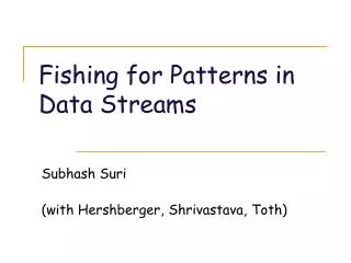
Fishing for Patterns in Data Streams Subhash Suri (with Hershberger, Shrivastava, Toth)
2 9 9 9 7 6 4 9 9 9 3 9 N = 12; item 9 is majority An Old Chestnut: Majority • A sequence of N items. • You have constant memory. • In one pass, decide if some item is in majority (occurs > N/2 times)?
Misra-Gries Algorithm (‘82) • A counter and an ID. • If new item is same as stored ID, increment counter. • Otherwise, decrement the counter. • If counter 0, store new item with count = 1. • If counter > 0, then its item is the only candidate for majority.
ID ID1 ID2 . . . . IDk count . . A generalization: Frequent Items Find k items, each occurring at least N/(k+1) times. • Algorithm: • Maintain k items, and their counters. • If next item x is one of the k, increment its counter. • Else if a zero counter, put x there with count = 1 • Else (all counters non-zero) decrement all k counters
Frequent Elements: Analysis • A frequent item’s count is decremented if all counters are full: it erases k+1 items. • If x occurs > N/(k+1) times, then it cannot be completely erased. • Similarly, x must get inserted at some point, because there are not enough items to keep it away.
Data Stream Algorithms • Majority and Frequent are examples of data stream algorithms. • Data arrives as an online sequence x1, x2, …, potentially infinite. • Algorithm processes data in one pass (in given order) • Algorithm’s memory is significantly smaller than input data • Summarize the data: compute useful patterns
Streaming Data Sources • Internet traffic monitoring • Web logs and click streams • Financial and stock market data • Retail and credit card transactions • Telecom calling records • Sensor networks, surveillance • RFID • Instruction profiling in microprocessors • Data warehouses (random access too expensive).
Stream of IP-Packets Internet Traffic Analysis • Usage trends for engineering, provisioning, abuse detection, etc. • Discover sources of large traffic • Items = IP packets • Item ID = Flow ID • E.g. sender’s IP address • Frequent items = Heavy Hitters • E.g. report all flows that consume more than 1% of the link bandwidth. • Counting bytes, instead of number of occurrence.
Stream of IP-Packets Stream Data • Rapid, continuous arrival: • Several million packets/sec • Huge volume: • > 50 TB of header data per day for Gigabit router • Real time response • Small memory: fast but costly SRAM • In the sea of data, spot unusual traffic patterns and anomalies
Problem of False Positives • False positives in Misra-Gries algorithm • It identifies all true heavy hitters, but not all reported items are necessarily heavy hitters. • How can we tell if the non-zero counters correspond to true heavy hitters or not? • A second pass is needed to verify. • False positives are problematic if heavy hitters are used for billing or punishment. • What guarantees can we achieve in one pass?
Approximation Guarantees • Find heavy hitters with a guaranteed approximation error [Demaine et al., Manku-Motwani, Estan-Varghese…] • Manku-Motwani (Lossy Counting) • Suppose you want -heavy hitters--- items with freq > N • An approximation parameter , where << .(E.g., = .01 and = .0001; = 1% and = .01% ) • Identify all items with frequency > N • No reported item has frequency < ( - )N • The algorithm uses O(1/ log (N)) memory
Misra-Gries revisited • Running MG algorithm with k = 1/ counters also achieves the -approximation. • Undercounts any item by at most N. • In fact, MG uses only O(1/) memory. • Manku-Motwani slightly better in per-item processing cost • MG requires extra data structure for decrementing all counters: O(log(1/)) per item • Manku-Motwani is O(1) amortized per item. • See Demaine et al. for more details.
Patterns in Internet Traffic • No flow ID. • Knowledge of applications, connections etc. has to be inferred by analysis. • Raw stream data is too low level • Patterns are visible only in multi-dimensions. • Useful patterns require paying attention to Internet hierarchy.
Hierarchy in Data UCSB • An example IP address hierarchy. • We are interested in subgroups that emerge as heavy hitters. • Heavy hitter can be a single machine, or it can be formed by a group. • To avoid redundancy, a higher level entity should exclude a lower node already tagged as heavy. • Is CS a heavy hitter even without Web Server or only because of it? PHY CS GSL CSIL Lab1 CS WebServer
Dimensions in Data • IP Packets can be summarized along multiple dimensions: src, dst, protocol, ports, etc. • Useful patterns may involve multiple dimensions. • Aggregation by IP src identifies servers; aggregation by ports identifies applications. • To learn which servers generate which kind of traffic requires fishing on both fields simultaneously. Src1 DestIP B Dest1 C A Subnet2 WebServer Subnet1 SrcIP
A geometric formulation • A stream of points • E.g. IP packets in header space • Set of implicitly defined boxes • Patterns or classification rules • A box B is heavy if it contains > N points. • Discounted frequency of B: exclude the points that are in heavy boxes properly contained in B. • Hierarchical Heavy Hitters: a box is a -HHH if its discountedfrequency > N B A C Discounted Frequency C
Computing HHH • The number of -HHHs is at most A/, where A is size of largest anti-chain in the hierarchy. • Max number of overlapping but incomparable boxes. • Assume constant. • Estan-Savage-Varghese (sigcomm ‘03): • Offline: require multiple passes • Do not find true HHHs: difficulty of overlapping boxes • Heuristic optimizations: first find 1D heavy hitters and then do the cross product for multidim-HHH, etc. • Cormode et al. (vldb ‘03, sigmod ‘04): • Extends Lossy Counting (Manku-Motwani) algorithm • Heuristics to deal with overlap problems • Online and space-efficient, but no bounds on discounted freq
Discounted frequency Problem • No existing space-efficient scheme offers a provable guarantee on the discounted frequency • Worst-case bounds hold only for total freq • Thus, the problem of false positives. • Two sources of problem: • Loss of information during merges • Overlapping boxes C C B B A A
Complexity of HHHs • Can we have provable guarantees just like flat heavy hitters? • Guaranteed separation between heavy and non-heavy boxes • Every box identified as -HHH should have discounted frequency > N • All other boxes have discounted frequency < ( - ) N • Hershberger-Shrivastava-Suri-Toth [PODS 05] • Any -HHH algorithm with fixed approximation guarantee in d-dim must use W(d+1) memory in worst-case.
The Lower Bound in 1-D • r intervals of length 2 each (call them literals) • Union of the r intervals is B. • Each interval split into two unit length sub-intervals. • If stream points fall in the left (resp. right) subinterval, we say the literal has orientation 0 (resp. 1). B 2r Literal 0 1
The Construction • Stream arrives in 2 phases. • In 1st phase: • Put 3N/r points in each interval, either in left or right half. • In 2nd phase • Adversary chooses either left or right half for each sub-interval and puts N points. Call these intervals sticks. • Heavy hitters: • Each stick is a -HHH • Discounted frequency of B (the union interval) depends on literals whose orientations in 1st and 2nd phase differ Algorithms must keep track of W(r) orientations after 1st phase B
The Lower Bound • Suppose an algorithm A uses at most 0.01r bits of space. • After phase 1, it encodes orientations of the r literals in 0.01r bits. • There are 2r distinct orientation • Two orientations that differ in at least r/3 literals map to the same (0.01r)-bit code ==> indistinguishable to A. • If orientations in 1st and 2nd phase are same, frequency of B = 0, not a HHH. • If r/3 literals differ, frequency of B = r/3 * 3N/r = N, so B is -HHH • So, A misclassifies B in one sequence. B
Completing the Lower Bound 2r • Make r independent copies of the construction • Use only one of them to complete the construction in the 2nd phase • Need O(r2) bits to track all orientations • For r = 1/4, this give W(-2)lower bound B r
Multi-dimensional lower bound • The 1-D lower bound is information-theoretic; applies to all algorithms. • For higher dimensions, need a more restrictive model of algorithms. • Box Counter Model. • Algorithm with memory m has m counters • These counters maintain frequency of boxes • All deterministic heavy hitter algorithms fit this model • In the box counter model, finding -HHH in d-dim with any fixed approximation requires W(d+1) memory
0 1 Literal Diagonal Uniform Stick 2r 2D (Multi-Dim) Construction • A box B and a set of descendants. • B has side length 2r. • 1st phase • 2x2 (literal) boxes in upper left quadrant (orientation 0 or 1) • 2nd phase • Diagonal: boxes in upper left quadrant; all orientation 0 • Sticks: 1xr (or rx1) boxes • Uniform: lower right quadrant
FullyCovered Half Covered Multi-dimensional lower bound • Intuition: • Each stick combines with a diagonal box to form a skinny -HHH box • Diagonal boxes pair-up to form -HHH • Skinny boxes form a checker-board pattern in upper left quadrant • Each literal is either fully covered or half covered • As in 1-D, adversary picks sticks • Discounted frequency of B has • Half covered literals and • Points in the Uniform quadrant Diagonal Uniform Stick 2r
The Lower Bound • The algorithm must remember the W(r2) literal orientations. • Otherwise, it cannot distinguish between two sequences, where discounted frequency of B is m or 3m/2, resp. (for m = 20/29 N). • Like before, by making r copies of the construction, we get the lower bound of W(r3). • The basic construction generalized to d dimensions. • Adjusting the hierarchy to get lower bound for any arbitrary approximation
Hierarchical Heavy Hitters • In the most general setting, no space-efficient scheme may be possible for -HHH with guaranteed approximation quality. • W(d+1) memory in worst-case. • Some tractable summaries: Adaptive Spatial Partitioning; Median and Quantiles; Geometric Summaries.
Conclusions • Age of data glut. • Growing need for real time analytics. • Locality and geometric structures. • Which geometric patterns are hard to detect in streams? • Which data mining tasks are feasible in streams?