Download
1 / 40
400 likes | 526 Views
Stochastic Tractography Analysis of the uncinate fasciculus. Andrew Rausch Psychiatry Neuroimaging Laboratory Brigham & Women's Hospital rauscha@bwh.harvard.edu ∘ (617)-525-6118 NA-MIC Tutorial Contest: Summer 2010. Learning Objective.

E N D
Stochastic Tractography Analysis of the uncinate fasciculus Andrew Rausch Psychiatry Neuroimaging Laboratory Brigham & Women's Hospital rauscha@bwh.harvard.edu∘ (617)-525-6118 NA-MIC Tutorial Contest: Summer 2010
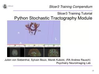
Learning Objective This tutorial will lead you through a Fractional Anisotropy analysis of the uncinate fasciculus to illustrate using the stochastic tractography module in Slicer 3.6 Visualized stochastic cloud of the uncinate fasciculus
Pre-requisite To use this tutorial, you should already know how to load images, create ROI labelmaps, and do basic work with diffusion MRI images. See especially the Visualization tutorial and the Diffusion tutorial by Sonia Pujol: http://www.slicer.org/slicerWiki/images/6/67/Slicer3Course_DataLoading_3DVisualization_SoniaPujol.pdf http://www.slicer.org/slicerWiki/images/2/20/DiffusionMRITutorial_SFN2009_SPujol.pdf
Material • This tutorial requires the installation of the Slicer3.6 release and the tutorial dataset. They are available at the following locations: • Slicer3.6 download page http://www.slicer.org/pages/Downloads/ • Tutorial dataset: stochastic_tutoral_data.zip [http://www.na-mic.org/Wiki/images/e/e7/Stochastic_tutorial_data.zip] Disclaimer:It is the responsibility of the user of Slicer to comply with both the terms of the license and with the applicable laws, regulations, and rules.
Platform This tutorial was developed on a 64-bit Linux operating system. It has been tested on no other systems at this time.
Overview Discussion Set up Slicer Running stochastic tractography Visualizing results Analyzing results Conclusion
How it works Stochastic tractography finds the probability of connection between a seeding region and another point This is done by calculating streamline tracts with a small amount of variation introduced at each step. These tracts are then averaged to produce a “stochastic cloud”
How it works Streamline tractography of the uncinate. Streamline shows direct connections between regions, allowing fiber based analysis of measures or analysis of voxels within the tract’s path. Note the thin, separate tracts. Stochastic shows the “probability” of connection, allowing weighted analysis of measures in the cloud. Note smooth, averaged cloud. Stochastic tractography of the uncinate.
Setting up The Stochastic Tractography module feeds data to python, where it does all its processing. You need to enable this by checking “Enable Slicer Daemon” in Slicer’s settings.
Setting up • Go to “View” -> “Application Settings” • Select “Slicer Settings” then • Check “Enable Slicer Daemon” • Now restart Slicer3 • This step only needs to be completed once
Setting up • Load the images in the dataset • DWI: A filtered and eddy current corrected diffusion weighted MRI • Mask: from Diffusion Tensor Estimation module • ROIA: labelmap slice of uncinate • ROIB: labelmap slice of uncinate DWI (baseline shown) Mask from Estimation module ROI A (shown over baseline) ROI B (shown over baseline)
Run Tractography It is now time to start Stochastic Tractography. You will find the module in: Modules -> Diffusion -> Tractography -> Stochastic Tractography There are a number of inputs and optional commands for the module. In the following slides we will cover which options to choose.
Run Tractography Here you pick the DWI image to use as well as the seeding and filtering ROIs, and a white matter volume to mask the tensor volume before tractography. • IO tab: • Input DWI Volume: DWI.nhdr • Input ROI Volume (Region A): ROIA.nhdr • Input ROI Volume (Region B): ROIB.nhdr • Input WM Volume: mask.nhdr
Run Tractography Here you will decide how to smooth the DWI image before estimating tensors. This will help to remove noise and improve the tracking algorithm. • Smoothing tab: • Enabled: check • Gaussian FWHM: “1.2,1.2,1.2”
Run Tractography Here you will decide threshold values for the brain mask, if you are using a B0 baseline image to do the masking instead of a supplied WM Volume. • Brain Mask tab: • Enabled: do not check. • Lower Brain threshold: N/A • Higher Brain Threshold: N/A
Run Tractography Here you supply whether your imaging is based on IJK coordinates or RAS. • IJK/RAS switch tab: • Enabled: check
Run Tractography Here you choose which diffusion measures you would like Slicer to calculate as it performs tractography • Diffusion Tensor tab: • Enabled: check • FA: check • TRACE: do not check • MODE: do not check
Run Tractography Here you set the parameters of stochastic tractography, total tracts means seed tracts per voxel, Max tract length cuts off fibers longer than value, step size is distance between tensor recalculation. We don’t use spacing or stopping criteria, and “basic method” refers to using the Friman algorithm for stochastic tractography. • Stopping criteria: do not check • FA: N/A • Use basic method: check • Tractography tab: • Enabled: check • Total Tracts: 500 • Maximum tract length: 200 • Step Size (mm): 0.8 • Use spacing: do not check
Run Tractography Here you set parameters for the creation of the connectivity map. Cumulative adds each tract passing though a voxel, length based removes tracts based on their size category, threshold sets a minimum probability threshold for showing, tract offset enlarges the target ROI, Use Spherical ROI vicinity creates a spherical target ROI, with size set by Vicinity. • Connectivity Map tab: • Computation Mode: cumulative • Length Based: N/A • Length Class: N/A • Threshold: N/A • Tract offset: N/A • Use spherical ROI vicinity: N/A • Vicinity: N/A
Run Tractography Here you enable the automatic start of the python server that does the processing. • Automatic Server Initialisation tab: • Enabled: check
Run Tractography Hit “Apply” to begin tractography A dialog prompting you to “allow incoming connections?” will appear. Select OK.
Run Tractography Data will now be sent to the python program, and you can watch the progress in the command line terminal. Completing the program takes a long time – on a 2.3GHz computer with 8GB RAM it runs for ~24 hrs.
Stochastic Output You will know the program has finished when the results appear in the scene. You can see by going to “Module” -> “Data.” • The following volumes appear when complete: • smooth • brain • tensor • fa • cmFA • cmFB • cmFAandB • cmFAorB
Stochastic Output • Smooth • If you enabled smoothing, this volume shows the results on a B0-baseline image.
Stochastic Output • Brain • This image shows the mask used. If you selected a WM Volume, this is it, if you set threshold values in the brain mask tab, this is the resulting brain mask.
Stochastic Output • Tensor • This is a tensor volume, estimated from a smoothed version of the DWI you provided. Here it is represented with a color by orientation map.
Stochastic Output • FA • This is fractional anisotropy volume, calculated from the tensor volume, above.
Stochastic Output • cmFA • This is a normalized connectivity map showing the probability of a voxel's connection to region A.
Stochastic Output • cmFB • This is a normalized connectivity map showing the probability of a voxel's connection to region B.
Stochastic Output • cmFAandB • This is a normalized connectivity map showing the intersection of the cmFA and cmFB maps.
Stochastic Output • cmFAorB • This is a normalized connectivity map showing the union of the cmFA and cmFB maps.
Visualize An easy way to visualize the stochastic cloud is through the “Volume Rendering” module – this will create a 3D model where opacity values of the cloud are assigned based on the probability. Higher probability means a denser cloud.
Visualize Under “Source” select “cmFAandB_somenumber” “Scenario,” “ROI,” and “Property” will all automatically populate.
Visualize The 3D model will appear in the 3D viewing window. From here you can adjust the background images shown as described in the basic tutorial.
Analyze As an example for the analysis of stochastic tractography results, we will count the mean FA covered by the tracts. We will first find all tracts with a greater than 10% chance of connection. Then we will weight the FA map by the probability of connection Finally, we will find the mean FA by use of the Label Statistics module.
Analyze • Threshold: • Select cmFAandB in “Background” • of one slice window • Go to “Modules” -> “Editor” • A window asking for your label map • selection will appear. Hit “OK” • Select the “Threshold” button • Change the threshold to 0.1-1 • Hit “Apply” • Every voxel in cmFAandB that was • above 0.1 should now be colored in • on the labelmap, cmFAandB_#####-label To analyze the outputs of stochastic tractography, we want to count the mean FA contained in the tracts. We will do this two ways: • Threshold: average FA for all voxels above the 0.1 (10%) probability of connection • Weighted: average FA in all voxels in the cloud, weighted by the probability of connection
Analyze To create a weighted FA volume for analysis, go to: “Modules” -> “Filtering” -> “Arithmetic” -> “Multiply images” IO Tab: Input Volume 1: fa Input Volume 2: cmFAandB Output Volume: Create New Volume Then, under Output Volume, select Rename and rename the volume “FA_multiplied” Controls Tab: Interpolation order: 1 Hit Apply
Analyze To get results, we will go to: “Modules” -> “Quantification” -> “Label Statistics” Input Grayscale Volume: FA_multiplied Input Labelmap: cmFAandB_#####-label Hit Apply. The results will appear in the spreadsheet below. Scroll to the right to see the average and standard deviation for FA under label 1 – all the voxels with a probability of over 0.1 You can save the results to a text document for further analysis with “Save to File”
Conclude We have now seen the complete process of running stochastic tractography from setting up Slicer to running stochastic tractography, to visualizing the results, and finally analyzing the outputs.
Acknowledgments National Alliance for Medical Image Computing NIH U54EB005149 Psychiatry Neuroimaging Laboratory of Brigham and Women’s Hospital Julien von Siebenthal for developing this module Doug Terry for writing an earlier version of this tutorial