GAs and Premature Convergence

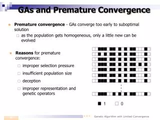
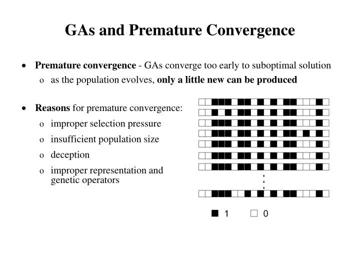
1. GAs and Premature Convergence • Premature convergence - GAs converge too early to suboptimal solution • as the population evolves, only a little new can be produced • Reasons for premature convergence: • improper selection pressure • insufficient population size • deception • improper representation and genetic operators

2. Motivation and Realization • Motivation – to maintain a diversity of the evolved population and extend the explorative power of the algorithm • Realization • Convergence of the population is allowed up to specified extent • Convergence at individual positions of the representation is controlled • Convergence rate – specifies a maximal difference in the frequency of ones and zeroes in every column of the population • ranges from 0 to PopSize/2 • Principal condition – at any position of the representation neither ones nor zeroes can exceed the frequency constraint • Specific way of modifying the population genotype

3. Algorithm of GALCO 1. Generate initial population 2. Choose parents 3. Create offspring 4. if (offspring > parents) then replace parents with offspring else{ find(replacement) replace_with_mask(child1, replacement) find(replacement) replace_with_mask(child2, replacement) } 5. if (not finished) then go to step 2

4. 50 Operator replace_with_mask Mask – vector of integer counters; stores a number of 1s for each bit of the representation

5. Testovací úlohy - statické • Deceptive function • F101(x, y) • Hierarchická funkce • Royal Road Problem

6. GALCO – vliv parametru C

7. GALCO vs. SGA

8. GALCO – vliv parametru C

9. GALCO vs. SGA

10. Multimodal Optimization Initial population SIGA with without

11. Multimodal Optimization (cont.) Initial population GALCO SIGA

12. GA s reálně kódovanou binární rep. (GARB) • Pseudo-binární rep.- bity kódovány reálným číslem r 0.0, 1.0 • interpretace(r) =1, pro r> 0.5 = 0, pro r < 0.5 redundance kódu • Příklad: ch1 = [0.92 0.07 0.23 0.62] ch2 = [0.65 0.19 0.41 0.86] interpretace(ch1) = interpretace(ch2) = [1 0 0 1] • Síla genů – vyjadřuje míru stability genů • Čím blíže k 0.5 tím je gen slabší (nestabilnější) • „Jedničkové geny“: 0.92 > 0.86 > 0.65 > 0.62 • „Nulové geny“: 0.07 > 0.19 > 0.23 > 0.41

13. Gene-strength adjustment mechanism • Geny chromozomů vzniklých při křížení jsou upraveny • v závislosti na jejich interpretaci • a relativní frequenci jedniček (nul) na dané pozici v populaci P[] př.: P[0.82 0.17 0.35 0.68]  v populaci je na 1. pozici 82% jedniček, na 2. pozici 17% jedniček, na 3. pozici 35% jedniček, na 4. pozici 68% jedniček. • Geny, které v populaci převládají jsou oslabovány; ostatní jsou posilovány.

14. Posilování a oslabování genů • Oslabování gen’ =gen+c*(1.0-P[i]), když (gen<0.5) a (P[i]<0.5) (gen má hodnotu nula a v populaci na i-té pozici převažují nuly) a gen’ = gen – c*P[i], když (gen>0.5) a (P[i]>0.5) • Posilování gen’ = gen – c*(P[i]), když (gen<0.5) a (P[i]>0.5) (gen má hodnotu nula a v populaci na i-té pozici převažují jedničky) a gen’ = gen + c*(1.0-P[i]), když (gen>0.5) a (P[i]<0.5) • Konstanta c určuje rychlost adaptace genů: c (0.0,0.2

15. Stabilizace slibných jedinců • Potomci, kteří jsou lepší než jejich rodiče by měli být stabilnější než ostatní vygenerovaná nekvalitní řešení • Chromozomy slibných jedinců jsou vygenerovány se silnými geny ch = (0.71, 0.45, 0.18, 0.57)  ch’= (0.97,0.03, 0.02, 0.99) • Geny slibných jedinců přežijí více generací aniž by byly zmeněny v důsledku oslabování

16. Pseudocode for GARB 1 begin 2 initialize(OldPop) 3 repeat 4 calculate P[] from OldPop 5 repeat 6 select Parents from OldPop 7 generate Children 8 adjust Children genes 9 evaluate Children 10 if Child is better than Parents 11 then rescale Child 12 insert Children to NewPop 13 until NewPop is completed 14 switch OldPop and NewPop 15 until termination condition 16 end

17. Testovací úlohy - dynamické • Ošmerův dynamický problém g(x,t) = 1-exp(-200(x-c(t))2) c(t) = 0,04(t/20) • Minimum g(x,t)=0.0 se mění každých 20 generací • Oscillating Knapsack Problem 14 objektů, wi=2i, i=0,...,13 f(x)=1/(1+target-wixi) • Target osciluje mezi hodnotami 12643 a 2837, které se v binárním vyjádření liší o 9 bitů

18. DF3 H-IFF F101 Výsledky na statických problémech F101

19. Výsledky na statických problémech

20. Výsledky na dynamických problémech Oscillating knapsack problem

21. MTE – Mean Tracking Error[%] – střední odchylka nejlepšího jedince v populaci a optimálního řešení počítaná přes všechny gen. Bezprostředně po změně opt. Celkově Algoritmus MTEStDevMTEStDev GARB c = 0:02583.330.650.425.2 GARBc = 0:07525.634.62.47.4 GARBc = 0:12512.822.41.03.9 GARBc = 0:17510.219.70.73.0 GARBc = 0:2259.219.30.62.7 SGA binaryN/AN/A57.343.61 SGA GrayN/AN/A47.6642.94 CBM-BN/AN/A19.3933.13 Výsledky na dynamických problémech • Ošmerův dynamický problém

22. Zotavení z homogenní populace

23. Weakness of Simple Selectorecombinative GAs • Scale poorely on hard problems, largely the result of their mixing behaviour • Inability of SGA to correctly identify and adequately mix the appropriate BBs in subsequent generations • Exponential computation complexity of SGA • Crossover operators or other exchange emchanisms are needed such that adapt to the problem at hand • Linkage adaptation

24. Naivní přístupy – operátor inverze • Obrátí pořadí genů náhodně vybraného podřetězce v chromozomu 10011 – (1,1) | (2,0)(3,0)(4,1) | (5,1) • po inverzi (1,1)(4,1)(3,0)(2,0)(5,1) • Nepoužitelné z důvodu nevyváženosti signálu pro zlepšování linkage oproti signálu pro učení allel. • tα< tλ - alely podstupují přímější selekci než linkage  GA se rozhodne pro optimální nastavení alel dříve než zjistí, které kombinace genů zformovat dohromady a vzájemně mixovat. • Řešení: obrátit nerovnítko na tα> tλ (ALE JAK?)

25. Competent GAs • Can solve • hard problems (multimodal, deceptive, high degree of subsolution interaction, noise, ...), • quickly, • accurately, • reliably. • Messy GAs – mGA, fmGA, gemGA • Learning linkage GAs – LLGA • Compact GAs – cGA, ECGA • Bayesian optimization algorithm - BOA

26. Messy Genetic Algorithms - mGAs • Inspirationfrom the nature – evolution starts from the simplest forms of life • mGA departed from SGA in four ways: • messy codings • messy operators • separation of processing into three heterogeneous phases • epoch-wise iteration to improve the complexity of solution

27. mGA’s codings • Tagged alleles: • Variable-length strings: (name1, allele1) … (nameN, alleleN) ((4,0) (1,1) (2,0) (4,1) (4,1) (5,1)) • Over-specification – multiple gene instances (gene 4) • Majority voting – would express deceptive genes too readily • First-come first-served (left to right expression) - positional priority • Underspecification – missing gene instances (gene 3) • Average schema value – variance is too high • Competitive template – solution locally optimal with respect to k-bit perturbations

28. Messy operators: cut & splice • Cut – divides a single string into two parts • Splice – joins the head of one string with the tail of the other one • When short strings are mated – probability of cut is small  mostly the string will be just spliced • the strings’ length is doubled • When long string are mated – probability of cut is large  one-point crossover

29. mGAs: three heterogeneous phases • Initialization • Enumerative initialization of the population with all sub-strings of a certain length k<<l (lk)2k O(lk) computations • Guaranteed that all BBs of certain size are present in the population • Primordial phase • Only selection used to dope the population with good BBs • Good linkage groups are selected before their alleles are allowed to be mixed • Juxtapositional phase • selection + cut&splice • Mixing of the BBs

30. Fast messy genetic algorithms - fmGAs • Probabilistically complete enumeration • Population of strings of length l’ close to l is generated • Assumption: each string contains many different BBs of length k<<l • Building block filtering – extracts highly-fit and effectively linked BBs • Repeated (1) selection and (2) gene deletion • Only O(l) computations to converge • Extended thresholding – tournaments are held only between strings that have a threshold number of genes in common • fmGA vs mGA: 150-bit long problem, 305-bit deceptive function • 1.9105 vs. 5.9108 evaluations

31. Gene expression messy GA - gemGA • Messy ??? • No variable-length strings • No under- or over-specification • No left-to-right expression • Messy use of heterogeneous phases of processing in gemGA • Linkage learning phase - first identifies linkage groups • Mixing phase – selection + recombination • exchanges good allele combinations within those groups to find optimal solution

32. gemGA: The idea • Linkage learning phase • Transcription I (antimutation) • Each string undergoes l one-bit perturbations • Improvements are ignored ?!? (bit does not belong to optimal BB) • Changes that degrade the structure are marked as possible linkage groups candidates Ex.: two 3-bit deceptive BBs 111 101 marked not marked (degrades) (improves) • Transcription II • Identifies the exact relations among the genes by checking nonlinearities IF f(X’i) + f(X’j) != f(X’ij) THEN link(i,j)

33. Linkage Learning GA - LLGA • More “messy” than gemGA • Variable-length strings • Left-to-right expression • Always over-specification • NO primordial or juxtapositional phase – more SGA like • Idea: • Probabilistic expression that slows down the convergence of alleles • Crossover that adapts linkage at the same time that alleles are exchanged

34. Clockwise interpretation  (3,1)(2,0)(5,1)(1,1)(4,0)  1 0 1 0 1 LLGA – Probabilistic expression

35. LLGA – probabilistic expression cont. • The allele 1 is expressed with the probability δ/l and 1/l respectively • The allele 0 is expressed with the probability (l-δ)/l and (l-1)/l respectively

36. LLGA: Effect of PE on BBs • Assume a 6-bit problem where BB requiring genes 4, 5, and 6 to take on values of 1 in a trap function. • Initially the block 111 will be expressed roughly 1/8th of the time • After the linkage evolved properly the BB success rate increases (6,1) (4,1) (5,1) (4,0) (5,0) (6,0) expressed most of the time almost never expressed • Extended probabilistic expression EPE-q • q is the number of copies of unexpressed allele (q=2)

37. LLGA – introns • Introns – non-coding genes (97% of DNA is non-coding) • Number of introns required for proper functioning grows exponentially  compressed introns

38. Probabilistic Model-Building GAs • Initialize population at random • Select promising solutions • Build probabilistic model of selected solutions • Sample built model to generate new solutions • Incorporate new solutions into original population • Go to 2 (if not finished)

40. 5-bit trap problem

41. UMDA performance

42. UMDA with “good” statistics

43. Extended compact GA - ECGA • Marginal product model (MPM) • Groups of bits (partitions) treated as chunks • Partitions represent subproblem • Onemax: [1] [2] [3] [4] [5] [6] [7] [8] [9] [10] • Traps: [1 2 3 4 5] [6 7 8 9 10]

44. Learning structure in ECGA • Two components • Scoring metrics: minimal description length (MDL) • Number of bits for storing probabilities: Cm = log2Ni 2Si • Number of bits storing population using model: Cp = NiE(Mi) • Minimize C = Cm + Cp • Search procedure: a greedy algorithm • Start with one-bit groups • Merge two groups for most improvement • No more improvement possible  finish.

45. ECGA model

46. ECGA example