Download
1 / 10
100 likes | 199 Views
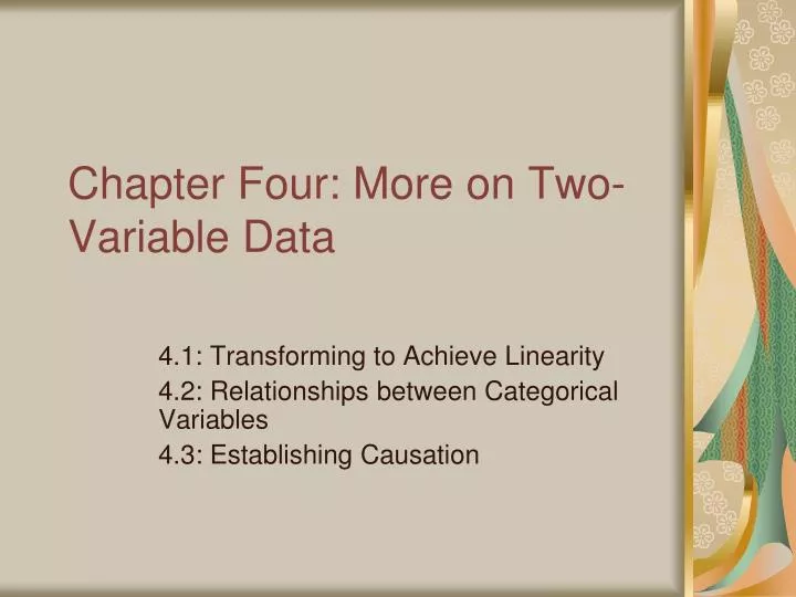
Chapter Four: More on Two-Variable Data. 4.1: Transforming to Achieve Linearity 4.2: Relationships between Categorical Variables 4.3: Establishing Causation. 4.1: Transforming to Achieve Linearity. Two specific types of nonlinear growth: An exponential function has the form y = ab x .

E N D
Chapter Four: More on Two-Variable Data 4.1: Transforming to Achieve Linearity 4.2: Relationships between Categorical Variables 4.3: Establishing Causation
4.1: Transforming to Achieve Linearity • Two specific types of nonlinear growth: • An exponential function has the form y = abx. • A power function follows the form y = axb. • To test if data follows linear or nonlinear growth, check the difference between consecutive y-values: • There is linear growth if a fixed amount is added to y for each increase in x. • The data is exponential if the common ratio, found using yn/yn-1, is equal between consecutive y-values. • If the common ratio > 1, exponential growth is occurring, and if the common ratio < 1, exponential decay is occurring. • Both exponential and power function equations use essentially the same format: • Transform into linear forms, use the linear regression to find the LSRL, and take an inverse transformation to get a curve modeling the original data.
Exponential Functions • Once you know that the data represents an exponential function, plug the data into your calculator. • Create a separate list for log(y) and use that information to derive the LSRL: • log ŷ = a + bx • To determine the linearity, check the correlation and residual plot. • The residual plot is the graph of x vs RESID. A pattern would indicate that a linear relationship is not the best model for the association of the variables. • Raise 10 to both sides of the equation (ie, take the inverse of log), and simplify: • 10log ŷ = 10a+bx • ŷ = (10a)(10bx) • This gives you the exponential form to fit the original data. • Graph the original scatterplot, and overlay with this equation as y = 10^(RegEQ)
Example • Electronic Funds Transfer (EFT) machines first appeared in the 1980s, and their use increased drastically in the years following. Look at the table on the following slide, and determine if the transactions grew exponentially. Then obtain the LSRL equation, and from that obtain the equation for the model.
Steps • 1—Graph initial data (x vs. y) • 2—Test for exponential growth (yn/yn-1) • 3—Perform linear regression on initial data • 4—Look at residual plot of initial data and consider r and r2 • 5—Transform y to log y • 6—Graph transformed data (x vs. log y) • 7—Perform linear regression on transformed data • 8—Look at residual plot, r, and r2 • 9—Perform inverse transformation of linear equation to arrive at exponential model • 10—Graph initial data with exponential model
Results • log ŷ = -.3481 + .0459x where ŷ is the predicted number of transactions in millions and x is the year since 1900 • r2 = .9979, r = .9990 • This tells us that our linear model above is a good fit for the transformed date and that our exponential model will be a good fit for the initial data. In particular, we can see that 99.79% of the variation in the log of transactions in millions can be explained by the linear relationship with the year. • ŷ = (10-.3481)(10.0459x)
Power Functions • Begin with the form y = axb. • Take the logarithm of both sides to obtain log y = (log axb), and simplify: • log ŷ = log a + (b log x) • This is a form of a linear equation, so the least-squares regression can be derived from it, with log x as the horizontal variable and log y as the vertical variable. • Further simplify the equation to obtain: • log ŷ = log a + log xb • To return to the original form, perform inverse transformation by raising 10 to each side of the equation, and simplify: • 10log ŷ = 10log a + log xb • 10log ŷ = 10log a + log xb • ŷ = (10log a)(10log xb) • = (10log a)(10log x)b • = (10log a)(xb) • = axb
Example • Using the following table for Olympic weightlifting records, determine if the data shows exponential growth or power regression, and determine the correlation of the LSRL. Then plot the residuals and transformed points, and find a new equation of best fit for the original scatterplot.