Blue: Histogram of normalised deviation from “true” value; Red: Gaussian fit to histogram

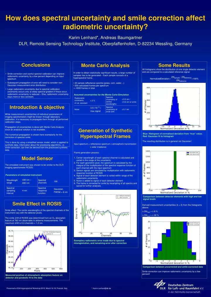
1. Monte Carlo Analysis • In order to obtain statistically significant results, a large number of samples has to be generated – Each sample consists of a hyperspectral frame. • 20 sample reflectance spectra (grass, corn, water…) • 200 calculated frames per spectrum • 4000 frames in total Assumed uncertainties for the Monte Carlo-Simulation Radiometric uncertainty of cal. standard ± 2 % Spectral uncertainty of central wavelengths ± 0.2 nm / ± 0.6 nm w/ smile Noise Spectral uncertainty of smile shift ± 0.1 nm • Smile correction and careful spectral calibration can improve radiometric uncertainty by a few percent depending on input spectrum • Subsequent propagation of error will need to consider non-Gaussian measurement error distribution • Large radiometric uncertainty due to spectral calibration uncertainty occurs only at steep spectral gradient If these occur, radiometric uncertainty is reduced – Else, radiometric uncertainty stays more or less constant. Introduction & objective While measurement uncertainties of individual parameters of imaging spectrometers might be known through laboratory calibration, it is necessary to propagate them through all performed calibration steps. Propagation of uncertainties is done with Monte Carlo Analysis since an analytical solution is not available. The numerical propagation is shown here exemplarily for the correction of spectral smile. This is done by using a simplified sensor model, which is applied to synthetic data. Information about the processing algorithms, i.e. smile correction, can then be derived from the processed synthetic data. Model Sensor The simulated instrument was chosen to be similar to the DLR imaging spectrometer ROSIS: Parameters of simulated instrument Wavelength range 430 nm – 830 nm Spectral channels 100 Spectral sampling interval 4 nm Spectral response function Gaussian, FWHM = 6 nm Conclusions Smile Effect in ROSIS Smile effect: The centre wavelengths of the spectral channels of the instrument vary with the detector pixels. The smile shift of ROSIS was determined from an O2 absorption feature at 762 nm observable in airborne measurements. The maximum shift is 0.3 channels = 1.2 nm. Measured position of atmospheric absorption feature on detector and parabolic fit to the data How does spectral uncertainty and smile correction affect radiometric uncertainty? Karim Lenhard*, Andreas Baumgartner DLR, Remote Sensing Technology Institute, Oberpfaffenhofen, D-82234 Wessling, Germany Some Results All histograms show the distribution of one single detector element and are compared to a calculated reference signal: Generation of Synthetic Hyperspectral Frames Blue: Histogram of normalised deviation from “true” value; Red: Gaussian fit to histogram The resulting distribution is in general not Gaussian! • Input spectrum = reflectance spectrum xatmospheric transmission • xsolar irradiance • Frame generation process: • Center wavelength of each spectral channel is calculated and varied in the range of the uncertainty • For each geometric pixel, the spectrum is calculated by the integral of the multiplication of the spectral response function of each channel with the input spectrum • Sensor signals are simulated by multiplication with radiometric response function of ROSIS • Signal of each detector element is varied within range of the radiometric uncertainty • Noise is added to signal of each detector element • The frame is corrected for smile by resampling of all spectra and saved for further analyses. Comparison between detector elements with high and low signal levels Derived measurement uncertainties (k = 2) from the histograms above: D DNHigh = ±8 % D DNLow = ±30 % Exemplary radiometric error made due to spectral misregistration, and remaining error after correction Comparison between uncorrected and smile-corrected data Smile correction can improve radiometric uncertainty by a few percent! Presented at ESA Hyperspectral Workshop 2010, March 16-19, Frascati, Italy *: Karim.Lenhard@dlr.de