Download
1 / 17
170 likes | 277 Views
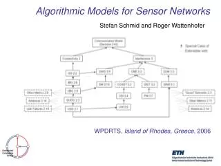
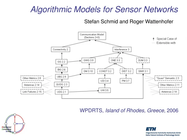
Algorithmic Models for Sensor Networks. Schmid, Wattenhofer IPDPS’06. Models and Sensor Networks. To develop algorithms and mathematically prove their correctness, simplifying models are needed for WSN’s.

E N D
Algorithmic Models for Sensor Networks Schmid, Wattenhofer IPDPS’06
Models and Sensor Networks • To develop algorithms and mathematically prove their correctness, simplifying models are needed for WSN’s. • Balance between simplifying the model in order to keep the analysis tractable and neglecting important properties of the nw • Common representations are as a graph, geometric representation.
Connectivity Models • Given a set of nodes, which nodes can recv the transmission of a given node • Is u adjacent to v ? • Typically symmetric. • Classic model UDG • Transmission range normalized to 1
UDG • Idealistic since real radios are not omni directional and even small obstacles affect connectivity • Proposed General Graph
Connectivity models (contd.) • Too pessimistic! • Something between the 2 extremes. • QDG with ρ=1 is a UDG
UDG to QUDG • Many algorithms can be transformed from UDG to QUDG at a cost of 1/ρ2 • This ok for ρ=0.5 (4) • But for ρ=0.1, much worse (100) • Still does not translate nicely to obstacles like walls – eg. All nodes on one side of the wall can talk to each other but not the opposite side
Extending the dimension • 2d • Nodes in 2d Euclidean plane form a doubling metric • General graph does not
Additional variations • Antennas variations besides omni-directional • Link failures – model probabilistically
Interference • Important for lower layer protocols • Most popular: SINR Signal to Noise Interference Ratio • Does not specify power. 3 ways:
Interference • The SINR model is very complicated • A lot of far away transmissions sum up as noise to a sender-receiver pair • ONE is popular. UDG with one – UDI shown next
Algorithms • Global – can operate on entire network • Distributed – a node has information about only its own state. Messages need to be exchanged to learn more about the nw. All nodes run their own algorithm • Localized – Special case of distributed. Limited to k. A node can retard its right to communicate i.e. some causality
Other assumptions • MAC – ideal vs. interference (adversary) • Random node distribution – uniform distribution in 2d plane. Also Poisson • Worst-case node distribution – completely arbitrary • Node id’s – again worst, random. Range can limit also
Other assumptions • Location info: absolute or relative to other nodes. • Sleep time energy consumption • Lifetime definitions.
Conclusion • No one model • Emphasized that for correctness, the more pessimistic or conservative models should be used • Broad overview provided.