Download
1 / 8
80 likes | 172 Views
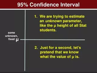
More about the Confidence Interval of the Population Mean. Remember looking at the normal table? Sure you do!

E N D
Remember looking at the normal table? Sure you do! Let’s look at some z’s. A z=1.96 gives a tabled value of .9750. The number .9750 is the area under the curve to the left of z and would be the areas a, b, and c added up. Now area d = 1-.9750 = .025. Since the graph is symmetric, area a is also .025. Thus, and this is an important point, area b and c = .95 or 95% Not the greatest graph a b c d Sample means
Okay, since we know (by a rule called the central limit theorem) the center of the sampling distribution of sample means is the population mean, if we go out from the mean 1.96 standard errors in both directions then we will have 95% of the sample means. The area in the graph labeled a and d adds up to .05. The confidence interval looks in the middle, but we could also talk about the “tails” on both ends of the distribution. The .05 is called the alpha value, or the level of significance and is the probability that the interval estimation procedure will not contain the population mean. More about this later. But some more terminology: Alpha = .05 goes along with a 95% confidence interval. Alpha divided by 2 would be the value in each tail of the distribution.
Remember at the beginning of a previous section I had an example about the sprinkler in my front yard? I said if the sprinkler is in the middle I will cover 95% of the yard with the water. Then I had you place the sprinkler in the yard at night after I spun you around (this is to simulate a random process) and we said you would get the middle wet 95% of the time. (Sometimes you would actually water my neighbors driveway, and as my neighbor said once, “the driveway will not grow much”) Now back on slide two I had two arrows at the bottom of the graph, one in each direction. The arrow is of a certain length – like how far the water shoots out from the sprinkler in each direction – and by analogy the length is 1.96 times the standard error.
Now I need you to be active here. The distribution below is a theory about all the means from samples of a given size we could take. But we only take 1 sample. We have a 95% chance our 1 sample mean is in area b, c. Here is the active part: choose any value in b, c by marking it with a pencil on the number line and call this your sample mean – I put an x below. Now imagine you can pick up the two arrows and place them down by the x – I have the faded arrows. Do my arrows cover the center? Yes! This will happen with a 95% probability. There is only a 5% chance my sample mean will be in a or d and thus the arrows will not cover the center. Not the greatest graph a b c d x Sample means
Now I have said round z to 2 decimals when you need to calculate a z. I still mean this. But look at the z’s 1.64 and 1.65. The areas in the table are .9495 and .9505. So, a z =1.645 would have an area to the left =.9500 and a tail area = .05. Alpha = .1 here and we would have a 90% confidence interval. Not the greatest graph Sample means
Look at the z’s 2.57 and 2.58. The areas are .9949 and .9951. Then you would think a z=2.575 would have an area = .9950. Well the process is not exactly linear, so the convention is to say a z = 2.576 would have an area to the left = .9950 and thus a tail area =.005. Our book just says use 2.58 here! Alpha would be .01 and the confidence interval would be 99%. Let’s turn to a problem to drive these points home, OKAY? Not the greatest graph Sample means
Problem 2 page 245 Here I put a number line and we do not know the population mean, just the sample mean. X bar = 125 The interval will use a Z of 2.58 with a 99% interval. Thus we use the value 2.58(24)/sqrt(36) = 2.58(24)/6 = 2.58(4) = 10.32. Thus the lower limit of our interval is 125 – 10.32 = 114.68 and the upper limit is 135.32 and we report the interval as either (114.68, 135.32) or 114.68 ≤ μ ≤ 135.32.