Download
1 / 69
690 likes | 890 Views
Resolution Enhancement in MRI. By: Eyal Carmi Joint work with: Siyuan Liu , Noga Alon, Amos Fiat & Daniel Fiat. Lecture Outline. Introduction to MRI The SRR problem (Camera & MRI) Our Resolution Enhancement Algorithm Results Open Problems. Introduction to MRI.

E N D
Resolution Enhancementin MRI By: Eyal Carmi Joint work with: Siyuan Liu, Noga Alon, Amos Fiat & Daniel Fiat
Lecture Outline • Introduction to MRI • The SRR problem (Camera & MRI) • Our Resolution Enhancement Algorithm • Results • Open Problems
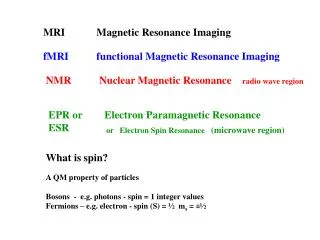
Introduction to MRI • Magnetic resonance imaging (MRI) is an imaging technique used primarily in medical settings to produce high quality images of the inside of the human body.
Introduction to MRI • The nucleus of an atom spins, or precesses, on an axis. • Hydrogen atoms – has a single proton and a large magnetic moment.
MagneticResonance Imaging • Uniform Static Magnetic Field – Atoms will line up with the direction of the magnetic field.
MagneticResonanceImaging • Resonance – A state of phase coherence among the spins. • Applying RF pulse at Larmor frequency • When the RF is turned off the excess energy is released and picked up.
z x y MagneticResonance Imaging • Gradient Magnetic Fields – Time varying magnetic fields (Used for signal localization)
MagneticResonance Imaging • Gradient Magnetic Fields: 1-D Y B0 B1 B2 B3 B4 X
B1(t) ω2 FT ω1 z1 z2 z3 z4 Signal Localization slice selection • Gradient Magnetic Fields for slice selection ω Gz,1 Gz,2 z
B0 Gx(t) t Signal Localizationfrequency encoding • Gradient Magnetic Fields for in-plane encoding x B=B0+Gx(t)x t
B0 Gx(t) t Signal Localizationphase encoding • Gradient Magnetic Fields for in-plane encoding x B=B0+Gx(t)x t
y 1-D path Wy Δkx Wx x k-space interpretation k-space DFT Sampling Points
MagneticResonanceImaging Collected Data (k-space) 2-D DFT
The Super Resolution Problem Definition: SRR (Super Resolution Reconstruction): The process of combining several low resolution images to create a high-resolution image.
SRR – Imagery Model • The imagery process model: • Yk – K-th low resolution input image. • Gk – Geometric trans. operator for the k-th image. • Bk – Blur operator of the k-th image. • Dk – Decimation operator for the k-th image. • Ek – White Additive Noise.
SRR – Main Approaches • Frequency Domain techniques Tsai & Huang [1984] Kim [1990] Frequency Domain
Back Projection Current HR Best Guess Back Projected LR images Original LR images Iterative Refinement SRR – Main Approaches • Iterative Algorithms Irani & Peleg [1993] : Iterative Back Projection
SRR – Main Approaches • Patti, Sezan & Teklap [1994] POCS: • Elad & Feuer [1996 & 1997] ML: MAP: POCS & ML
SRR – In MRI • Peled & Yeshurun [2000] 2-D SRR, IBP, single FOV, problems with sub-pixel shifts. • Greenspan, Oz, Kiryati and Peled [2002] 3-D SRR (slice-select direction), IBP.
Resolution Enhancement Alg. • A Model for the problem • Reconstruction using boundary values • 1-D Algorithm • 2-D Algorithm
Modeling The Problem • Subject Area: 1x1 rectilinearly aligned square grid. (0,0)
Modeling The Problem • True Image : A matrix of real values associated with a rectilinearly aligned grid of arbitrary high resolution. (0,0)
Modeling The Problem • A Scan of the image: Pixel resolution – Offset – True Image Image Scan, m=2
Modeling The Problem • Definitions: Maximal resolution – Pixel resolution = Maximal Offset resolution – • We can perform scans at offsets where with pixel resolution
Modeling The Problem • Goal: Compute an image of the subject area with pixel resolution while the maximal measured pixel resolution is • Errors: 1. Errors ~ Pixel Size & Coefficients 2. Immune to Local Errors => localized errors should have localized effect.
0 C 0 C 0 C 0000 CCC Using boundary value conditions • Assumption: or Reconstruct using multiple scans with the same pixel resolution. • Introduce a variable for each HR pixel of physical dimension . • Algorithm: Perform c2 scans at all offsets & Solve linear equations (Gaussian elimination). 0 C
Using boundary value conditionsExample: 4 Scans, PD=2x2 Second sample
Using boundary value conditionsExample: 4 Scans, PD=2x2 0 0 0 0
Problems using boundary valuesExample: 4 Scans, PD=2x2 (0,0)
Problems using boundary valuesExample: 4 Scans, PD=2x2 (-1,-1)
Add more information • Solve using LS • Propagation • problem Problems using boundary valuesExample: 4 Scans, PD=2x2
???? ? ? ? ? ? ? ???? b x A Demands On the algorithm • No assumptions on the values of the true image. • Over determined set of equations Use LS to reduce errors: • Error propagation will be localized.
The One dimensional algorithm • Input: Pixel of dimension • Notation: gcd(x,y) – greatest common divisor of x & y. (Extended Euclidean Algorithm)
The One dimensional algorithm (Extended Euclidean Algorithm)
The One dimensional algorithm Algorithm: Given w.l.g, let: a>0 & b<0 To compute , compute:
The One dimensional algorithmLocalized Reconstruction Localized Reconstruction Effective Area: x+y high-resolution pixels
Two and More Dimensions • Given pixels of size: Where x,y & z are relatively prime. Reconstruct 1x1 pixels. • Error Propagation is limited to an area of O(xyz) HR pixels. Stack 1-D Algorithm
Two and More Dimensions gcd(xy,xz)=x gcd(xy,zy)=y 1-D Algorithm
Example Two dimensional reconstruction PD=5x5 PD=15x1 PD=3x3
Example Two dimensional reconstruction PD=4x4 PD=12x1 PD=3x3
Example Two dimensional reconstruction PD=5x5 PD=20x1 PD=4x4
Larger Dimensions Generalize to Dimension k Using k+1 relatively prime Low-Resolution pixels