Download

1 / 30
310 likes | 536 Views
f. Quantum infodynamics: An alternative approach to quantum theory of open systems. Vladimír Bužek. QGATES QUPRODIS QUEST. The First QuICT Network Meeting , Abingdon, UK, 1 1 – 13 July 200 3. M otivation. Information encoded in a state of a quantum system

E N D
Quantum infodynamics: An alternative approach to quantum theory of open systems VladimírBužek QGATES QUPRODIS QUEST The First QuICT Network Meeting , Abingdon, UK, 11 – 13 July 2003
Motivation • Information encoded in a state of a quantum system • The system interacts with a large reservoir • The system “decays” into an “equilibrium” state • Where the original information goes ? • Is the process reversible ? • Can we recover diluted information ? • Can we introduce a master equation?
Physics of information transfer System S - a single qubit initially prepared in the unknown state ReservoirR - composed of N qubits all prepared in the state , which is arbitrary but same for all qubits. The state of reservoir is described by the density matrix . InteractionU- a unitary operator.We assume that at each time step the system qubit interacts with just a single qubit from the reservoir. Moreover, the system qubit can interact with each of the reservoir qubits at most once. R.Alicki & K.Lendi, Quantum Dynamical Semigroups and Applications, Lecture Notes in Physiscs (Springer, Berlin, 1987) U.Weiss, Quantum Dissipative Systems (World Scientific, Singapore, 1999) B.M.Terhal & D.P.diVincenzo, Phys. Rev. A 61, 022301 (2001).
4s 2s 0s 1s 3s Quantum Homogenization t =
Definition of quantum homogenizer • Homogenizationis the process in which is some distance defined on the set of all qubit states . At the output the homogenizerall qubits are approximately in a vicinity of the state . • Covariance No cloning theorem
Dynamicsof homogenization: Partial Swap Transformation satisfying the conditions of homogenization form a one-parametric family where S is the swap operator acting as The partial swap is the only transformation satifying the homogenization conditions
with MapsInduced by Partial Swap Thepartial swap U and the reservoir state induce a superoperator on the system If we introduce a trace distance we find that the transformation is contractive, i.e. for all states Banach theorem implies that for all states iterations converge to a fixed point of , i.e. to the state
Homogenization of Gaussian states • The signal is in a Gaussian state • Reservoir states are Gaussian without displacement • The signal after k interactions changes according to
0 1 2 4 6 8 10 12 Homogenization of Gaussian states II • Quantum homogenization– squeezed vacuum reservoir state signal state signal after interactions
Quantum homogenization– squeezed vacuum many 14 16 20 26 33 44 Homogenization of Gaussian states II reservoir state signal state signal after interactions
4s 2s 0s 1s 3s Entanglement due to homogenization t =
Homogenized qubits saturate the CKW inequality Entanglement: CKW inequality The CKW inequality V.Coffman, J.Kundu, W.K.Wootters, Phys.Rev.A61,052306 (2000)] The conjecture
Where the information goes? Initially we had and reservoir particles in state For large , and all N+1 particles are in the state Moreover all concurrencies vanish in the limit . Therefore, the entanglement between any pair of qubits is zero, i.e. Also the entanglement between a given qubit and rest of the homogenized system, expressed in terms of the function is zero. Information cannot be lost. The process is UNITARY !
Information in correlations Pairwise entanglement in the limittends to zero. We have infinitely many infinitely small correlations between qubits and it seems that the required information is lost. But, if we sum up all the mutual concurrencies between all pairsof qubits we obtain a finite value The information about the initial state of the system is “hidden” in mutual correlations between qubits of the homogenized system. Can this information be recovered?
Classical information has to be kept in order to reverse quantum process Reversibility Perfect recovery can be performed only when the N + 1 qubits of the output state interact, via the inverse of the original partial-swap operation, in the correct order.
Irreversibility If the order of the interaction between the system and the reservoir particles is not know If the reservoir particles are indistinguishable (different model – results are OK) Random trial – the probability of success P= 1/ (N+1)!
Stochastic homogenization I • Bipartite interaction : • Initial state of the system: • Reduced density matrix of the system after n interactions: Example of a stochastic evolution of the system qubits S with 10 qubits in the reservoir.
Comparison of deterministic and stochastic homogenization • Step in deterministic model vs. step in stochastic model • Probability of interaction of the system S in: • Deterministic model: • Stochastic model: Stochastic evolution of the system qubit S interacting with a reservoir of 100 qubits. The figure shows one particular stochastic evolution of the system S (red line), the deterministic evolution of the system S (blue line) and the average over 1000 different stochastic evolutions of the system S (pink line) Necessity of rescaling
Reversibility • Recovery of the initial state • “Spontaneous” recurrence - number of steps needed for 90% recovery is the system qubit S interacting a reservoir composed of 100 qubits one particular stochastic evolution of the system S (red line) up to 500 interactions
Master equation & dynamical semigroup • Standard approach (Davies) – continuous unitary evolution on extended system (system + reservoir) • Reduced dynamics under various approximations – dynamical continuous semigroup • From the conditions CP & continuity of dynamical semigroup can be written as • Evolution can be expressed via the generator • Lindblad master equation
Discrete dynamical semigroup • Any collision-like model determines one-parametric semigroup of CPTP maps • Semigroup property • Fundamental question: Can we introduce a continuous time version of this discrete dynamical semigroup?
From discrete to continuous semigroup • Discrete dynamics dynamical semigroup • We can derive continuous generalization - generator Decay time Decoherence time
Conclusions: Infodynamics • Dilution of quantum information via homogenization • Universality & uniqueness of the partial swap operation • Physical realization of contractive maps • Reversibility and classical information • Stochastic vs deterministic models • Lindblad master equation • Still many open questions Related papers: M.Ziman, P.Stelmachovic, V.Buzek, M.Hillery, V.Scarani, & N.Gisin, Phys.Rev.A65 ,042105 (2002)] V.Scarani, M.Ziman, P.Stelmachovic, N.Gisin, & V.Buzek, Phys. Rev. Lett. 88, 097905 (2002). D.Nagaj, P.Stelmachovic, V.Buzek, & M.S.Kim, Phys. Rev. A 66, 062307 (2002) M.Ziman, P.Stelmachovic, & V.Buzek, Fort. der Physik (2003); J. Opt. B (2003) + under preparation
Quasi-stationary limit • Average one-particle initial state: • In the case ofreservoir of 100 particles: • Corresponding limit of homogenization: Average over stochastic evolutions. The figure shows the average over stochastic evolutions of the system (dash-dotted line) with the average over the corresponding stochastic evolutions of one of the reservoir objects (dashed line) and the deterministic evolution (solid line)