Download
1 / 45
450 likes | 567 Views
Price Of Anarchy: Routing. Lecturer: Yishay Mansour Ido Trivizki and Mille Gandelsman. Routing – Lecture Overview. Optimize the performance of a congested and unregulated network: Network. Rate of traffic between each pair of nodes. Latency function.

E N D
Price Of Anarchy: Routing Lecturer: Yishay Mansour Ido Trivizki and Mille Gandelsman
Routing – Lecture Overview • Optimize the performance of a congested and unregulated network: • Network. • Rate of traffic between each pair of nodes. • Latency function. • Selfish behavior does not perform as well as an optimized regulated network. • Investigating the price of anarchy (PoA) by exploring the characteristics of Nash Equilibrium and mininal latency optimal flow.
Lecture overview – cont. • We will prove that: • If the latency of each edge is a linear function, PoA is at most 4/3. • In atomic routing the PoA is bounded by 2.6. • I the latency function is known to be continuous, non-decreasing and differentiable, there is no bounded coordination ratio.
Introduction • Job scheduling, discussed last time, can be viewed as a private case of routing. • Each player has to choose exactly one line to pass his traffic through. • Parallel lines routing:
Introduction – cont. • Today – the problem of routing traffic in a network: • Given a rate of traffic between pairs of nodes in the network, find an assignment of the traffic to paths so that the total latency is minimized. • It is often impossible to impose regulation, so we are interested in those settings where each user selects his minimum latency path: • Non-cooperative game in which each player plays best response – expect the routes to form a Nash Equilibrium.
Two player models • Non-atomic: we can split up traffic to several paths. • Atomic: each user chooses a single path on which he transports all of his traffic. The global target function in both cases is to minimize the total latency suffered by all users.
Reminder: The Price of Anarchy • The ration between the worst value of an equilibrium and that of the optimal: • Where OPT denotes the minimum latency among all feasible flows and C(x) is total cost of flow x. • Our goal is to bound the PoA.
Example 1: routing on parallel lines • n players with weights • m lines with speeds • The players are allowed to split their flow between different lines. • Nash Equilibrium is achieved when the load on each line is:
Example 1 – cont.Routing on parallel lines • The optimum is achieved by dividing the flow equally between the lines. • Therefore – we achieve a PoA=1
T S Example 2:Pigou’s Network • Nash flow will only traverse in the lower path. • OPT will divide the flow equally among the two paths. C(x)=1 C(x)=x
Example 2 – cont. • The target function is and it reaches minimum with value ¾, when x=1/2, giving a PoA of 4/3. • Combing the example with the tighter upper bound to be shown, it is a demonstration of a tight bound of 4/3 for linear latency functions.
C(x)=1 T S Example 3:Pigou’s Non-Linear Network • The flow at Nash will continue to use only the lower path.
Example 3 – cont. • Let (1-x) be the flow on the upper path in the optimum solution, and x - the flow on the lower path, respectively. • The overall cost is . • Proof that : • if we choose :
Example 3 – summary • In this case • It means that the PoA cannot be bounded from above in some cases when nonlinear latency functions are allowed.
Example 4 – Braess’s paradox • There are exactly two disjoint paths from s to t, each of them follows exactly two edges.
Example 4 – cont. • The optimal flow coincides with the Nash equilibrium: • half of the traffic takes the upper path, and the half the lower. • The latency perceived by each user is 3/2. • In any other non-equal distribution, there will be a difference in the total latency. • Users will be motivated to reroute to the less congested path.
Example 4 – cont. • Consider adding a fifth edge with latency 0. • The optimal flow stays 3/2. • Nash will only occur by routing the entire traffic on the single svwt path.
Example 4 – cont. • The latency each user experiences increases to 2. • Amazingly, adding a new zero latency link had a negative effect for all agents.
Formal Definition of the Problem • Consider a directed graph • Input: • k pairs of source and destination vertices • Demand ( the amount of required flow between and ). Assume: . • Each edge is given a load dependant non decreasing and differentiable latency function • Output: • Flow - a function that defines for each path a flow . induces flow on edge :
Formal Definition – cont. • We denote the set of simple paths connecting the pair by and let . • Solution is feasible if . • The latency of the a path is defines as: • Our goal is to find a flow that will minimize the total social cost of a flow is defined as: • The cost of player :
Flows at Nash equilibrium • Lemma: • A feasible flow for instance is Nash Equilibrium if for every and • Corollary: • is a flow at Nash Equilibrium for instance if and only if , where
Optimal Solution – flow • Our goal is find a feasible flow that will minimize the total cost. • Let . • Clearly, it follows that • To find the optimal flow , we will look at . • We assume that for each edge : is convex and therefore is also convex. • is differentiable.
The Optimality Condition • Define: and • Let be a dividable game. For each edge the function is convex, continuous and differentiable function. A flow is optimal for if and only if:
The Optimality Condition – cont. • Notice the resemblance between the characterization of optimality conditions and Nash Equilibrium. • An optimal flow can be interpreted as a Nash Equilibrium with respect to a different edge latency functions. • We will use this resemblance to reach the bound on PoA. • Where OPT denotes the minimum latency among all feasible flows and C(x) is total cost of flow x. • Our goal is to bound the PoA.
The Optimality Condition – cont. • Let: • Corollary: • is an optimal flow for if and only if it is Nash Equilibrium for the instance • Proof: • By the optimality condition: is optimal for if and only if , if and only if (by def.) , if and only if is Nash Equilibrium for .
The optimality condition - proof • Definition: a set is called a convex set if • Intuitively it means that a set is convex if the linear segment connecting two points in the set, is entirely in the set.
The optimality condition - proof • Definition: a function is called convex function if
The optimality condition - proof • Let be a convex function, and a convex set. • A convex programming is of the form: • Lemma: • If is strictly convex, then the solution is unique. • Proof: • Assume that are both minimum solutions. • Let , because is convex: . • Since is strictly convex: , contradicting and being minimal .
The optimality condition - proof • Lemma: • If is convex, then the solution set is convex. • Lemma: • If is convex and is not optimal then is not a local minimum. Consequently, any local minimum is also a global minimum. • Proof: • Assume that is not optimal, i.e. let , Since is convex: for every .
Existence of flows at Nash Equilibrium • Theorem: For every splittable game • There exists at least one Nash Equilibrium • If and are Nash equilibria then for every ,
Existence of flows at Nash Equilibrium - Proof • Define: , so that • Further define a potential function: • is non-negative, monotonous, increasing and differential. Is a convex function. • Nash equillibrium flows are global minimizers of
Existence of flows at Nash Equilibrium – Proof Cont. • By Weierstrass’s Theorem, has a minimum, and therefore Nash equilibrium exists. • Let and be Nash equillibria: • Define • and minimize , and we get • is sum of convex functions, and therefore it’s possible only if all members of the sum are equal, and therefore:
Bounding the Price of Anarchy • Theorem: If there exists a constant such that then • Corollary: If the latency function is polynomial function of degree , then
A tight bound for linear latency functions • A natural example for such a model: Network with congestion control (e.g.: TCP) • Using the corollary, we get a bound of 2 • We’ll show a bound of 4/3 (which is tight, as we’ve seen in Example 2) • When , both Nash and OPT (equal) will route all the flow in the shortest paths.
A tight bound for linear latency functions - Proof • Lemma (proof is trivial and omitted): • is a flow at Nash equilibrium, and is an optimal flow. Given a flow let
Unsplittable (Atomic) Routing • Example 1: • 4 players, all with demand 1 (r = 1): (U,V), (U,W), (V,W), (W,V) • An optimal and Nash equilibrium flow would use only edges with at total cost of 4
Unsplittable (Atomic) Routing – Exmaple 1 Cont. • Example 1 (cont.): • But the optimal solution is not the only NE. • Another Nash equilibrium: Player 1: U->W->V; Player 2: U->V->W; Player 3: V->U->W; Player 4: W->U->V With total cost of 10, which gives PoA = 2.5.
Unsplittable (Atomic) Routing – Exmaple 2 • Both players have s=S and t=T, but, player 1 has r=1, While player 2, r=2. • Possible paths S->T: p1: S->T; p2: S->V->T; p3: S->W->T; p4: S->V->W->T
Unsplittable (Atomic) Routing – Exmaple 2 Cont. • In this example there is no pure equilibrium. • Easy to show the following facts: • If player 2 chooses p1 or p2, player 1 will choose p4. • If player 1 chooses p4, player 2 will choose p3. • If player 2 chooses p3 or p4, player 1 will choose p1. • If player 1 chooses p1, player 2 will choose p2.
Unsplittable (Atomic) Routing – Existence of Nash Equilibrium • We’ve shown that NE does not always exist. • Theorem: If is an unsplittable game with then there exists a Nash equilibrium. • Proof: Define a potential function When player I moves from p to p’:
Unsplittable (Atomic) Routing – Existence of Nash EquilibriumCont. And: So: So when the players plays “best response” the potential decreases, and as it’s non-negative, s series of “best responses” will converge to a Nash equilibrium.
Bounding the price of anarchy for unsplittable linear games • Theorem: let be an unsplittable routing game with linear cost functions, then • Proof: • Let be a nashequillibirim (we assume it exists) flow, and be an optimal flow.
Bounding the price of anarchy for unsplittable linear games – Cont. • Lemma: • Proof (of lemma): • Using Cauchy-Schwartz:
Bounding the price of anarchy for unsplittable linear games – Cont. • We get: • Solving the equation for We get :