Download
1 / 61
610 likes | 723 Views
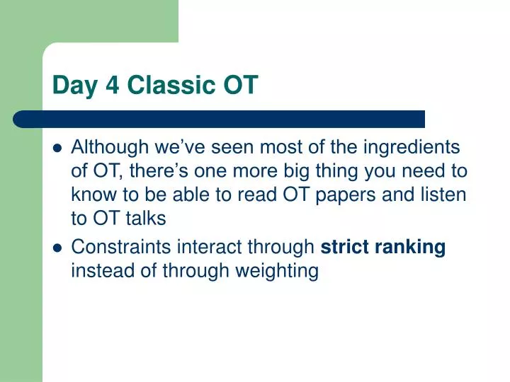
Day 4 Classic OT. Although we’ve seen most of the ingredients of OT, there’s one more big thing you need to know to be able to read OT papers and listen to OT talks Constraints interact through strict ranking instead of through weighting. Analogy: alphabetical order. Constraints

E N D
Day 4 Classic OT • Although we’ve seen most of the ingredients of OT, there’s one more big thing you need to know to be able to read OT papers and listen to OT talks • Constraints interact through strict ranking instead of through weighting
Analogy: alphabetical order • Constraints • HaveEarly1stLetter • HaveEarly2ndLetter • HaveEarly3rdLetter • HaveEarly4thLetter • HaveEarly5thLetter • ...
Harmonic grammar • Cabana wins because it does much better on less-important constraints
Classic Optimality Theory • Strict ranking: all the candidates that aren’t the best on the top constraint are eliminated • “!” means “eliminated here” • Shading on rest of row indicates it doesn’t matter how well or poorly the candidate does on subsequent constraints
Classic Optimality Theory • Repeat the elimination for subsequent constraints • Here, the two remaining candidates tie (both are the best), so we move to the next constraint • Winner(s) = the candidates that remain
“Harmonically bounded” candidates • A fancy term for candidates that can’t win under any ranking • Simple harmonic bounding: What can’t (c) win under any ranking?
“Harmonically bounded” candidates • Joint harmonic bounding: What can’t (c) win under any ranking?
Why this matters for variation • “Multi-site” variation: more than one place in word that can vary • Which candidates can win under some ranking?
Why this matters for variation • Even if the ranking is allowed to vary, candidates like (b) and (c) can never occur
How about in MaxEnt? • Can (b) and (c) ever occur?
How about in Noisy Harmonic Grammar? • Suppose the two constraints have the same weight
Summary for harmonic bounding • In OT, harmonically bounded candidates can never win under any ranking • means that applying a change to one part of a word but not another is impossible • In MaxEnt, all candidates have some probability of winning. • In Noisy HG, harmonically bounded candidates can win only in special cases. • See Jesney 2007 for a nice discussion of harmonic bounding in weighted models.
Is it good or bad that (b) and (c) can’t win in OT? • In my opinion, probably bad, because there are several cases where candidates like (b) and (c) do win...
French optional schwa deletion • There’s a long literature on this. See Riggle & Wilson 2005, Kaplan 2011 Kimper 2011 for references. • La queue de ce renard no deletion • La queue d’ ce renard some deletion • La queue de c’ renard some deletion • La queue de ce r’nard some deletion • La queue d’ ce r’nard as much deletion as possible, without violating *CCC
Pima plural marking • Munro & Riggle 2004, Uto-Aztecan language of Mexico, about 650 speakers [Lewis 2009]. • Infixing reduplication marks plural. • In compounds, any combination of members can reduplicate, as long as at least one does: Singular: [ʔus-kàlit-váinom], lit. tree-car-knife ‘wagon-knife’ Plural options: ʔuʔus-kàklit-vápainom ‘wagon-knives’ ʔuʔus-kàklit-váinom ʔuʔus-kàlit-vápainom ʔus-kàklit-vápainom ʔuʔus-kàlit-váinom ʔus-kàklit-váinom ʔus-kàlit-vápainom
Simplest theory of variation in OT: Anttila’s partial ranking (Anttila 1997) • Some constraints’ rankings are fixed; others vary • I’m using the red line here to indicate varying ranking
Anttilan partial ranking Max-C Ident(place) *θ Ident(continuant) *Dental
Linearization • In order to generate a form, the constraints have to be put into a linear order • Each linear order consistent with the grammar’s partial order is equally probable grammar linearization 1 (50%) lineariztn 2 (50%) Max-C Max-C Max-C Ident(place) Ident(place) Id(place) *θ Ident(cont) Ident(cont) *θ *θ Id(cont) *Dental *Dental *Dental [t̪ɪk] [θɪk]
Properties of this theory • No learning algorithm, unfortunately • Makes strong predictions about variation numbers: • If there are 2 constraints, what are the possible Anttilan grammars? • What variation pattern does each one predict?
Finnish example (Anttila 1997) • The genitive suffix has two forms • “strong”: -iden/-iten (with additional changes) • “weak”: -(j)en (data from p. 3)
Factors affecting variation • Anttila shows that choice is governed by... • avoiding sequence of heavies or lights (*HH, *LL) • avoiding high vowels in heavy syllables (*H/I) or low vowels in light syllables (*L/A)
Anttila’s grammar (p. 21) (Without going through the whole analysis)
Day 4 summary • We’ve seen Classic OT, and a simple way to capture variation in that theory • But there’s no learning algorithm available for this theory, so its usefulness is limited • Also, predictions may be too restrictive • E.g. if there are 2 constraints, the candidates must be distributed 100%-0%, 50%-50%, or 0%-100%
Next time (our final day) • A theory of variation in OT that permits finer-grained predictions, and has a learning algorithm • Ways to deal with lexical variation
Day 4 references • Anttila, A. (1997). Deriving variation from grammar. In F. Hinskens, R. van Hout, & W. L. Wetzels (Eds.), Variation, Change, and Phonological Theory (pp. 35–68). Amsterdam: John Benjamins. • Jesney, K. (2007). The locus of variation in weighted constraint grammars. In Workshop on Variatin, Gradience and Frequency in Phonology. Presented at the Workshop on Variatin, Gradience and Frequency in Phonology, Stanford University. • Kaplan, A. F. (2011). Variation Through Markedness Suppression. Phonology, 28(03), 331–370. doi:10.1017/S0952675711000200 • Kimper, W. A. (2011). Locality and globality in phonological variation. Natural Language & Linguistic Theory, 29(2), 423–465. doi:10.1007/s11049-011-9129-1 • Lewis, M. P. (Ed.). (2009). Ethnologue: languages of the world (16th ed.). Dallas, TX: SIL International. • Munro, P., & Riggle, J. (2004). Productivity and lexicalization in Pima compounds. In Proceedings of BLS. • Riggle, J., & Wilson, C. (2005). Local optionality. In L. Bateman & C. Ussery (Eds.), NELS 35.
Day 5: Before we start • Last time I promised to show you numbers for multi-site variation in MaxEnt • If weights are equal:
Day 5: Before we start • As weights move apart, “compromise” candidates remain more frequent than no-deletion candidate
Stochastic OT • Today we’ll see a richer model of variation in Classic (strict-ranking) OT. • But first, we need to discuss the concept of a probability distribution
What is a probability distribution • It’s a function from possible outcomes (of some random variable) to probabilities. • A simple example: flipping a fair coin
Probability distributions over grammars • One way to think about within-speaker variation is that, at each moment, the speaker has multiple grammars to choose between. • This idea is often invoked in syntactic variation (e.g., Yang 2010) • E.g., SVO order vs. verb-second order
Probability distributions over Classic OT grammars • We could have a theory that allows any probability distribution: • Max-C >> *θ >> Ident(continuant): 0.10 (t̪ɪn) • Max-C >> Ident(continuant) >> *θ:0.50 (θɪn) • *θ >> Max-C >> Ident(continuant): 0.05 (t̪ɪn) • *θ >> Ident(continuant)>> Max-C: 0.20 (ɪn) • Ident(continuant) >> Max-C >> *θ:0.05(θɪn) • Ident(continuant) >> *θ >> Max-C: 0 (ɪn) • The child has to learn a number for each ranking (except one)
Probability distributions over Classic OT grammars • But I haven’t seen any proposal like that in phonology • Instead, the probability distributions are usually constrained somehow
Anttilan partial ranking as a probability distribution over Classic OT grammars Id(place) *θ Id(cont) means • Id(place) >> *θ >> Id(cont): 50% • Id(place) >> Id(cont) >> *θ: 50% • *θ>> Id(place) >> Id(cont): 0% • *θ>> Id(cont) >> Id(place): 0% • Id(cont) >> *θ>> Id(place): 0% • Id(cont) >> Id(place) >> *θ: 0%
A less-restrictive theory: Stochastic OT • Early version of the idea from Hayes & MacEachern 1998. • Each constraint is associated with a range, and those ranges also have fringes (margem), indicated by “?” or “??” p. 43
Stochastic OT • Each time you want to generate an output, choose one point from each constraint’s range, then use a total ranking according to those points. • This approach defines (though without precise quantification) a probability distribution over constraint rankings.
Making it quantitative • Boersma 1997: the first theory to quantify ranking preference. • In the grammar, each constraint has a “ranking value”: *θ 101 Ident(cont) 99 • Every time a person speaks, they add a little noise to each of these numbers • then rank the constraints according to the new numbers. • ⇒ Go to demo [Day5_StochOT_Materials.xls] • Once again, this defines a probability distribution over constraint rankings • An Anttilan grammar is a special case of a Stochastic OT grammar
Boersma’s Gradual Learning Algorithm for stochastic OT • Start out with both constraints’ ranking values at 100. • You hear an adult say something—suppose /θɪk/ →[θɪk] • You use your current ranking values to produce an output. Suppose it’s /θɪk/ → [t̪ɪk]. • Your grammar produced the wrong result! (If the result was right, repeat from Step 2) • Constraints that [θɪk] violates are ranked too low; constraints that [t̪ɪk] violates are too high. • So, promote and demote them, by some fixed amount (say 0.33 points)
Gradual Learning Algorithm • demo (same Excel file, different worksheet)
Problems with the GLA for stochastic OT • Unlike with MaxEnt grammars, the space is not convex: there’s no guarantee that there isn’t a better set of ranking values far away from the current ones • And in any case, the GLA isn’t a “hill-climbing” algorithm. It doesn’t have a function it’s trying to optimize, but just a procedure for changing in response to data
Problems with GLA for stochastic OT • Pater 2008: constructed cases where some constraints never stop getting promoted (or demoted) • This means the grammar isn’t even converging to a wrong solution—it’s not converging at all! • I’ve experienced this in appyling the algorithm myself
Still, in many cases stochastic OT works well • E.g., Boersma & Hayes 2001 • Variation in Ilokano reduplication and metathesis • Variation in English light/dark /l/ • Variation in Finnish genitives (as we saw last time)
Type variation • All the theories of variation we’ve used so far predict token variation • In this case, every theory wrongly predicts that both words vary
Indexed constraints • Pater 2009, Becker 2009 • Some constraints apply only to certain words