Download
1 / 30
300 likes | 436 Views
Behaviours Of Cost Curves. Derivation And Properties of Short Run Total, Average And Marginal Cost Curves. How Does Total Cost Change ?.

E N D
Behaviours Of Cost Curves Derivation And Properties of Short Run Total, Average And Marginal Cost Curves
How Does Total Cost Change ? • It is actually a phenomenon in real world that as a firm increases its output, its productivity first rises faster and later rises much slower or even decreases. • So, if unit factor costs are kept constant, the total cost first rise relatively slower than the total output, but later rise much faster.
Why Does This Happen ? • In CE & AL level, such phenomenon is explained in short run by the Law of Diminishing (Marginal) Returns. • In long run, it is caused by the dominance of economies of scale in early production and diseconomies of scale later on.
Law of Diminishing Returns • This law states that when we continuously add variable factors to fixed factors, the total product (output) of a firm will first rise more than proportionally and then less than proportionally, or even decrease. • Alternatively, we say that the marginal product will eventually diminish.
An Illustration • Suppose a farmer has a piece of cultivated land and now wants to hire more workers to work on the farm. • Then he discovers that the farm’s output changes as follow:
Total product rises faster Total product rises slower Variable factor Fixed factor Output Table
Marginal product falls when the third worker is added. Output Table
Plotting Short Run Costs Curves • If factor costs are constant, e.g., the wage of hiring one more worker is no different from those hired before, total variable cost rises proportionally. • But due to the Law of Diminishing (Marginal) Returns, total product rises faster at first and slower later.
TVC Cost ($) Variable cost rises proportionally. TP(Q) TP rises faster at first but slower at the end.
Adding Fixed Cost • Fixed cost must occur as the production begins and will not change with total product. • In short run, the total cost of production includes both fixed and variable cost.
TC TVC TFC Total fixed cost is a horizontal line as it will not change with TP. Cost ($) TC and TVC are parallel because the vertical distance is fixed, that is the same as the fixed cost. TVC plus TFC will be TC. TP(Q)
TVC TVC1 TP1 TVC1 Ø TP1 Cost ($) = AVC1 = tan Ø As tan Ø increases when Ø is larger, AVC is also larger. TP(Q)
Q1 Q2 Q3 Cost ($) TVC Angle Ø decreases first and then rises. So does the AVC. TP(Q)
AVC Cost ($) AVC also falls at the beginning but rises later on. TP(Q) Q1 Q2 Q3
TC TVC Cost ($) At same Q, angle Ø for TC is greater than TVC. TP(Q) Q1 Q3
ATC AVC Cost ($) Thus, at same Q, ATC is higher than AVC. TP(Q) Q1 Q2 Q3
TFC TP TFC Cost ($) But for fixed cost, its average tends to fall as the total output increases. As only TP, not TFC, will increase, the average must be falling. = AFC TP(Q) Q1 Q3
AFC Cost ($) ATC and AVC are closing to each other because AFC is falling all the way. ATC AVC AVC plus AFC will be ATC TP(Q) Q1 Q2 Q3
TVC Ø> Ø’ Cost ($) The line from origin forms the lowest angel with TVC if it touches TVC, but not intersecting it. This tangency point means at Q’, we have the lowest AVC. Ø Ø’ TP(Q) Q’
TC Cost ($) The line from origin will touch TC at a higher Q than the TVC. TVC TP(Q) Q’ Q”
ATC AVC AFC Cost ($) ATC reaches minimum at a larger Q than the minimum AVC. TP(Q) Q’ Q”
ATC When AVC rises faster, ATC will rise. AVC When AFC falls faster, ATC still falls AFC TP(Q) Q’ Q” Cost ($) At the range Q’ to Q”, AVC is rising but AFC is falling.
Change in Total cost Change in Total Product Ø” This is a tangency line touching TVC. TVC Q1 Cost ($) Marginal cost = The tangency line will overlap the curve segment if the segment is very small. TP(Q)
Q1 Q2 Q3 Cost ($) TVC MC = AVC MC < AVC MC > AVC TP(Q)
AVC MC MC AVC Cost ($) MC < AVC MC > AVC MC = AVC TP(Q) Q1 Q2 Q3
MC AVC Cost ($) MC falls and rises faster than the AVC. When MC is smaller than AVC, AVC falls. MC cuts AVC’s minimum. TP(Q) Q1 Q2 Q3 When MC is larger than AVC, AVC falls.
TC TVC Q1 Q2 Cost ($) Slopes are equal for the same Q. TP(Q) So, only one MC for both TC and TVC, since they are parallel.
Q’ Q” Cost ($) TC MC also cuts TC’s minimum. TVC TP(Q)
MC ATC AVC AFC Q’ Q” MC cuts both ATC and AVC at their minimum. Cost ($) Assembly of all short run cost curves TP(Q)