Download
1 / 21
210 likes | 314 Views
Chi-Square Analysis. Basic Concepts, Section 13.2 Testing the Independence of Two Variables, Section 13.4. The Chi-Square Distribution. Let the random variable X be normally distributed with mean and standard deviation

E N D
Chi-Square Analysis Basic Concepts, Section 13.2 Testing the Independence of Two Variables, Section 13.4
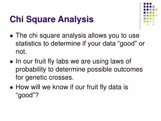
The Chi-Square Distribution • Let the random variable X be normally distributed with mean and standard deviation • Draw a large number of independent random samples of size n from this population and standardize each value x • Let the sample size be n = 2 • Draw our first sample • x1 and x2 • Standardize each value • Square the standardized value • Add over all observations within each sample PP 11
The Chi-Square Distribution • Draw a second sample of two observations and repeat the calculations • Since we have drawn a large number of such samples, we can create the sampling distribution of the statistic, which is the chi-square distribution PP 11
The Chi-Square Distribution • The distribution is skewed and its shape depends solely on the number of degrees of freedom • As the number of degrees of freedom increase, the distribution becomes more symmetrical • For this theoretical distribution, the degrees of freedom equal the number of independent squares of Z • In the preceding problem, with n = 2, the degrees of freedom = 2 • The domain of the chi-square distribution is restricted to non-negative real numbers = df = df = df = df As df becomes larger, curve approaches the normal distribution PP 11
Chi-Square Table • The chi-square table provides information on percentile points of the chi-square distribution for different degrees of freedom • The table shows the value of chi-square that will be exceeded only % of the time • If we had 15 degrees of freedom and we wanted to know the chi-square value that is exceeded only 5% of the time, we select as .05 in the top row and 15 degrees of freedom in the left most column and read the table entry as 24.9958 PP 11
Chi-Square Table • Notice that the entries begin with .99, .975, .95 • If we want to find the chi-square value that has only 5% of values less than it, we would look up the chi-square value that is exceeded 95% of the time • For 15 degrees of freedom, this value = 7.261 PP 11
Test for Independence • Think of a single sample being drawn from the population and that sample has two attributes • The hypothesis here is that one attribute is independent of another • The data in such hypotheses are often presented in a tabular form, and the table is called a contingency table • The contingency table has c (or k) columns and r rows and so we refer to it as a c by r contingency table • The data are either grouped data or nominal scale data • Nominal data means that we use numbers for the purpose of identifying groups, each number represents a category PP 11
Test for Independence • Test whether January is dependent on whether stock prices will go up or down in the entire year • The null hypothesis is that whether or not stock prices go up or down in the year is independent of whether they go up or down in January • H0: Stock price movements in the entire year is independent of stock price movements in January • H1: Stock price movements in the entire year is dependent of stock price movements in January • Gather data for 40 stocks in January and over the year and categorize their price movements as up or down PP 11
Observed Data • If the null hypothesis was true and these outcomes were independent, what would be the expected frequencies? PP 11
Definitions of Independence • (1) A and B are independent events if P(A|B) = P(A) • (2) The multiplication rule is used to find the probability of events A and B both occurring P(A B) = P(A|B) * P(B) • If we know events A and B are independent then we can substitute equation 1 into equation 2: • P(A B) = P(A) * P(B) PP 11
Independence • Let event A = January prices go up • Let event B = the year prices go up • P(Jan. up year up) = P(Jan. up) * P(Year up) • P(Jan. up year up) = 23/40 * 28/40 = .575 * .70 = .4025 • .4025 (40) = 16.1 expected number of stocks whose price went up in Jan and in the year PP 11
Independence • P(Jan. up Year down) = P(Jan. up) * P(Year down) • P(Jan. up Year down) = 23/40 *12/40 = .575 * .30 = .1725 • .1725 * 40 = 6.9 PP 11
Independence • A simple formula • where nr = the number of observations in the row • nc = the number of observations in the column • n = the total number of observations in the problem PP 11
Independence • For example ( 28*17)/40 = 11.9 • Notice that 16.1 + 6.9 = 23 • That is, the sum of the expected frequencies equals the sum of the observed frequencies • We can use this relationship (constraint) to calculate the one remaining expected value • In this 4 x 4 contingency table, we need to calculate only 2 of the four cells, • The remaining two can be figured out by subtraction PP 11
The Hypothesis Is That One Attribute Is Independent of Another • To test the null hypothesis, compare the frequencies which were observed with the frequencies we expect to observe if the null hypothesis is true • If the differences between the observed and the expected are small, that supports the null hypothesis • If the differences between the observed and the expected are large, we will be inclined to reject the null hypothesis PP 11
Test Statistic for Independence • The test statistic is Where r = number of rows in the contingency table k = number of columns in the table Oij = observed frequency in row i, column j Eij = expected frequency in row i, column j df = (r - 1)(k - 1) PP 11
Test Statistic • The test statistic is distributed approximately as a chi-square statistic • What does that mean? • Suppose the null hypothesis was correct and the two attributes are independent • If we were to repeatedly draw samples from the population, calculate the test statistic each time and then set up the distribution of the statistic, our statistic would follow the chi-square distribution PP 11
Problem with Stocks • In this problem, df = (r-1)(k-1) = 1 • r = 2, k = 2 • Looking at the chi-square table for df =1 • Only 5% of the time would we observe a test statistic greater than 3.84 • Only 1% of the time would we observe a test statistic greater than 6.635 • We consider these to be small probabilities. • When we observe a test statistic that would only occur 5% (or 1%) of the time when the null hypothesis is true, we reject the null hypothesis PP 11
Critical Values of Chi-Square, df = 1 Sampling Distribution of Test Statistic When Null Hypothesis is True • Calculated Test Statistic PP 11
Stock Problem • Statistical Decision • Reject the null hypothesis at 5% level of significance or at a 1% level of significance • Conclusions • Based on this evidence the probability that stock prices will go up during the entire year does not seem to be independent of whether or not they go up in January PP 11
Qualifications • The test should not be used when one or more of the expected frequencies is less than 5 • Alternatively, no cell should have an expected count less than one and no more than 20% of the cells should have an expected count less than 5 PP 11