Download
1 / 52
540 likes | 688 Views
Adaptive Portfolio Managers in Stock Market: An Approach Using Genetic Algorithms. K.Y. Szeto. Introduction Data Preprocessing Results of GA as a Forecasting Tool Portfolio Management Summary. Introduction. Complex System The Analysis of Stock Market

E N D
Adaptive Portfolio Managers in Stock Market: An Approach Using Genetic Algorithms K.Y. Szeto
Introduction • Data Preprocessing • Results of GA as a Forecasting Tool • Portfolio Management • Summary
Introduction • Complex System • The Analysis of Stock Market • Modify the Traditional Economic Models • Model the Individual Investor • Forecast Financial Time Series
Complex System • Stock market is an ideal complex system for investigations by financial analysts. • The laws underlying the dynamics are not even proven to exist. • Even if the underlying laws of economics trends are known, there is no way to predict the elusive human behavior. • As the complex system evolves, the “underlying laws” should also evolve along, albeit at a slower time scale.
The Analysis of Stock Market • Computer Programs • A given set of investment rules, extracted from historical data of the market. • Rules based on fundamental analysis or news obtained from the inner circle of the trade. • Statistical Results
Modify the Traditional Economic Models • To incorporate a certain level of communication among traders. (human interactions) • Mean Field Theory • Heterogeneous agents (psychological response) • different rules of investment • different human characters
Mean Field Theory • Each trader will interact with the average trader of the market, who is representative of the general atmosphereof investment at the time.
General Atmosphere • Model the general atmosphere of the market • We do not deduce it from a model of microscopic interaction between agents, but rather by a source of random news that serves as a kind of external, uncontrollable stimulus to the market. • Quantitative Parameters to measure individual characteristics of the trader, so that the response to the general atmosphere of the market is activated according to these parameters.
The Individual Investor • A rule of investment • Supplement the agent with specific value and character, representing the human psychology of a particular subset of investors. • Endow him/her with a particular skill of technical analysis.
Forecast Financial Time Series • Max (The rate of correct prediction) s.t. (A set of constrains) set by past patterns • Prediction is transformed into a problem of pattern recognition. • The data can be preprocessed using standard signal processing techniques.
Data Preprocessing • The signal processing techniques used here is mainly for the purpose of noise reduction and not for prediction, and no attempt is made on the theory behind the trend. • Transform a time series of rational numbers into one of alphabets or integers. • Divide the data with N points into two parts.
Transform a Time Series • Use a vector quantization technique to encode the time series as a sequence of integers corresponding to q classes. • For a given q, the original data set of N points will be divided into q sets, withN1, …,Nqmembers respectively. • For q=2 • Large fluctuation as class 1 • Small fluctuation as class 0 • For q=2m+1
Fluctuation • The fluctuation of the input {X'(t)} is computed as the fractional change in each interval. (The daily rate of return)
For q=2m+1, one can put down 2m boundary values{y-m, …, y0, ym}for q levels of fluctuations, such that • |y(t)| y0, X(t)=0 ?? • y0 y(t) y1 , X(t)=1 • y-1 y(t) y0, X(t)= -1 • we convert a time series into an integer sequence of data {X(t)} defined on the alphabets A’{-m,…,0,…,m} • Rename the q classes with the alphabets A{0, 1, …, q-1}
The Choice of the Boundary Values • Maximize the signal to noise ratio. • Set N1=N2= …=Nq • This criterion imposes a strict constraint on the boundary values, but the results will ensure a more precise comparison on the performance of the prediction tools on each class. • Adopt those normally used by traders on the daily rate of return to achieve immediate application.
Divide the Data • Training Set:M-L strings of length equal to L digits, along with the known associated action unit of each string. • Test Set:(N-M-L) sets of strings of length L, but the action unit should be used for performance evaluation. • The choice of L is important and one method is to use information entropy.
Results of GA as a Forecasting Tool • Generation of Time Series • Forecasting of Artificial Time Series • Forecasting of Real Financial Time Series • Self Organizing Behavior in GA
Generation of Time Series • Inverse Whitening Transformation • :diagonalizable nxn matrix • =diag[1,…,n] • eigenvector matrix =[1,…,n] • = • Using T= 1/2 T, the correlation matrix of Y=TX can be shown to be the identity matrix if the covariance matrix of the random variable X is .
Our first step is to generate an independent, normally distributed random variable Y with zero mean and unit variance. • Then we define the covariance matrix , which is a Toeplitz matrix with entries Cij=Cji=C(|i-j|). • It is a real symmetric matrix with unit diagonal and the function C(|i-j|) is related to the correlation function with given memory structure.
If the required time series has a short memory, one assumes an exponentially decaying function for these elements Cn=C(n)=exp(-n/). • is the range of correlation • n is the number of days in the past • The final result is a random variable x=T-1Y with correlation given by the covariance matrix .
Forecasting of Artificial Time Series • Three sets of short memory time series with 2000 data points are produced, with correlation functions C(n) with =5, 10, 15. • Training Set:first 1000 data points • cutoff values are used to put data points into five categories • Test Set:next 1000 data points
We want to maximize the correct percentage as well as the guessing percentage. • Specific rules:increase the correct percentage • General rules:increase the guessing percentage
In general the ratio of correct guess/total number of guess on the test set is around 50% to 60%. • For benchmark comparison with random guess, it gets a maximum of 20 % since there are 5 equally likely classes. • Another benchmark is random walk. It uses the value of previous time unit to predict the present unit. This method gives 25% of correct predictions. (See Table 1). ???
Table 1:Results of Prediction genetic algorithm performs best, especially in time series with long memory (larger time constant).
Forecasting of Real Financial Time Series • Experiment Setting • Two Benchmark Tests • Stock Price (Hang Seng Index) • Performance of Genetic Optimizer • The Performance of the Predictor • Probability of Correct Prediction
Experiment Setting • Training set:1712 data points • Test set:190 data points • Each experiment is started with different seed of random numbers. • 2000 generations • Repeated 15 times
Two Benchmark Tests • The first one is the random guess of two classes: stock prices go up and down with equal probability. • The second one is the random guess of two classes based on past statistics, in which case the probability of choosing 1 is 0.5144 and choosing 0 is 0.4856.
Performance of Self-Organized Genetic Optimizer 662.6+942.3<1712:sometimes no guess is made C0:the correct guess minus the wrong guess G0:the total number of guess made C1? G1?
The Performance of the Predictor • The average number of correct guess minus the wrong guess, which is the sum of C0 and C1. • Ideal Result:C0=110, C1=80, Sum=190 • Worst Case:C0=-80, C1=-110, Sum=-190 ?? ??
Probability of Correct Prediction • Pktest and Pktrain are the probability of correctly predicting the class k for the testing set and training set. • P0test=0.59, P1test=0.45, P0train=0.60, P1train=0.59 • The sum of probability of making a correct guess for both classes in the test set is 0.59+0.45=1.03, greater than one, an upper limit of any scheme of random guess.
Self Organizing Behavior in GA • A more important observation is the self-organizing behavior of the genetic optimizer without the Lagrange multipliers.
Suppose that the penalty of having too many or too few don't care bits compared to a chosen frequency (for example, 0.3) in the rules is not controlled by a Lagrange multiplier . • The exponent in the fitness controls the penalty, so that the fitness measure is modified by a factor of
Similarly, assume that the penalty of having a guessing frequency very different from the frequency of occurrence in the training set is not controlled by a Lagrange multiplier . • This exponent is to modify the fitness measure by a factor of
Then, these two factors will modify the expression of fitness by
Hk is independent of the rule index i so that it is a positive constant for the population of rules. • A new variable • If 1+ is positive, then fik is a monotonic function of . • Thus we can forget about Hk and use for our new fitness.
Portfolio Management • The level of confidence reflects the probability of change of the original strategy of investment, which is based on hard work on past data. • The degree of greed reflects the relative portion of each asset involved in each transaction, which definitely affects the final outcome of the investment. • Response to News and Level of Confidence • Level of Greed • Portfolio Management in the Presence of News
Response to News • “News” • A randomly generated time series • Take some kind of average of many real series of news. • An internally generated series that reflect the dynamics of interacting agents • For an agent who had originally forecasted a drop in the stock price tomorrow and planned to sell the stock at today's price, may change his plan after the arrival of the “good” news, and halt his selling decision or even convert selling into buying.
Four Scenarios • News is good and he plans to sell. • News is good and he plans to buy. • News is bad and he plans to sell. • News is bad and he plans to buy. re-evaluate re-evaluate
Level of Confidence • f:the level of fear • 1-f:the level of confidence • If f is 0.9, then the agent has 90% chance of changing his decision when news arrives that contradicts his original decision.
Choose a random number p. • If p > f, he will maintain his prediction, otherwise he reverses his prediction from 1 to 0 or from 0 to 1. • The bigger the value of f, the smaller the chance the random number p will be greater than f, implying that the smaller the chance he will maintain his original prediction.
Level of Greed • For a greedy investor, he may be very aggressive in all his investment, while a prudent investor will be more conservative in his action. • g:characterize the percentage of asset allocation in following a decision to buy or sell. • If g is 0.9, it means that the agent will invest 90% of his asset in trading. • g can be interpreted as a measure of greed.
Portfolio Management in the Presence of News • Training set • 800 points • Extract a rule using standard GAs. • Test set • 100 points • Evaluate the performance of the set of rules obtained after training. • News set • 1100 points • Investigate the performance of investors with different degree of greed and confidence.
x(t):the daily rate of return of a chosen stock • x(t) is a function of the value at x(t-1), x(t-2),..., x(t-k). Here k is set to 8. • Min MSE (to find a set of {i}) • |x(t)|1, |i|1, i=1,…,k
>0,the agent predicts an increase of the value of the stock. • 0, the agent predicts either an unchanged stock price or a decrease. • Count the guess as a correct one if the sign of the guess value is the same as the actual value, otherwise the guess is wrong. • If the actual value is zero, it is not counted.
Performance index Pc: • Pc=Nc/(Nc+Nw) • Nc is the number of correct guess • Nw is the number of wrong guess • While most investors make hard decision on buy and sell, the amount of asset involved can be a soft decision.
The final set of agents, all with the same chromosome (or rule), but with different parameters of greed g and fear f. • Initial Asset • Cash:10,000 USD • Shares:100 (at $99 a share) • The value of f and g ranged from 0 to 0.96 in increment of 0.04 will be used to define a set of 25x25=625 different agents.
Final Net Asset Values in Cash Greedy and confident investors perform better.
Summary • We construct a learning classifier system based on genetic algorithm. • Transform the problem of forecasting time series into a pattern recognition problem. • It performs better than both the random guess and random walk method on artificial data as well as real data. • This is superior to the use of Lagrange method for implementing constraints in the statistical properties of the rules.