Download

1 / 45
450 likes | 634 Views
Chapter 2. Nodes, Ties , and Influence. March 2013 Youn-Hee Han http://link.koreatech.ac.kr. 2.1 Importance of Nodes. Question: “ which nodes are important ” among a large number of connected nodes?

E N D
Chapter 2.Nodes, Ties, and Influence March 2013 Youn-Hee Han http://link.koreatech.ac.kr
2.1 Importance of Nodes • Question: “which nodes are important” among a large number of connected nodes? • Centrality analysis can provides answers with measures that define the importance of nodes • Different Centrality Analysis • a) Centrality based on the degree information of a node • Degree Centrality • Eigenvector (or Spectral) Centrality • b) Centrality based on the geodesic (i.e., shortest path) of nodes • Closeness Centrality • BetweennessCentrality
2.1 Importance of Nodes • Degree Centrality • Importance of a node is determined by the number of nodes adjacent to it • High-degree nodes naturally have more impact to reach a larger population than other nodes within the same network • Degree Centrality • Normalized Degree Centralitywhere n is the number of nodes in a network
2.1 Importance of Nodes • Degree Centrality • Degree centrality of v1 is 3 • Normalized degree centrality of v1 is 3 / (9-1) = 3/8
2.1 Importance of Nodes • Closeness Centrality • It measures how close a node is to all the other nodes • It describes the efficiency of information propagation from a node to all the others • It involves the computation of the average distance of one node to all the other nodes • Closeness Centralitywhere n is the number of nodes, and g(vi, vj) denotes the geodesic distance between nodes viand vj .
2.1 Importance of Nodes • Closeness Centrality • Closeness centrality of v3 and v4 • We conclude that v4is more central than v3.
2.1 Importance of Nodes • BetweennessCentrality • It measures the number of shortest paths in a network that will pass a node. • Nodes with high betweenness play a key role in the communication within the network • Betweenness centrality of a node • where • is the total number of shortest paths between nodes and • is the number of shortest paths between nodes and that pass along the node.
2.1 Importance of Nodes • Betweenness Centrality • σ19 = 2 1-4-5-7-9 and 1-4-6-7-9 • σ19(4) = 2, and σ19(5) = 1 • CB(4) = 15 • all shortest paths from {1, 2, 3} to {5, 6, 7, 8, 9} have to pass v4 • CB(5) = 6 • All the shortest paths from node {1, 2, 3, 4} to nodes {7, 8, 9}have to pass either v5 or v6 • Betweenness centrality of all nodes
2.1 Importance of Nodes • Betweenness Centrality • Maximum value of CB(vi) in an undirected network with n nodes • Normalized betweennesscentrality 6 1 7 2 CB(v5) = 8 * 7 / 2 = 28 5 8 3 9 4
2.1 Importance of Nodes • Eigenvector Centrality • A node’s importance is defined by its adjacent nodes’ importance. • Conceptually, • Let x denote the eigenvector centrality from v1 to vn. Then, the above equation can be written as in a matrix form • Equivalently, we can writewhere λ is a constant • It follows that • Thus x is an eigenvector of the adjacency matrix A.
2.1 Importance of Nodes • Eigenvector Centrality • How to get the top eigenvector xof the adjacency matrix A? • Transition matrix = Column-Normalized Adjacency Matrix • Transition matrix is constructed based on the adjacency matrix by normalizing each column to a sum of 1: • An entry ijdenotes the probability of transition from vj to vi = =
2.1 Importance of Nodes • Eigenvector Centrality • How to get the top eigenvector xof the adjacency matrix A? • It can be computed by the power method • i.e., repeatedly left-multiplying a non-negative vector xwith • x will be converged =
2.1 Importance of Nodes • Algorithmic Complexity • Degree centrality & Eigenvector centrality Low Complexity • Closeness centrality & Betweenness centrality High Complexity • For large-scale networks… • Efficient computation of centrality is critical and requires further research • Summary
2.2 Strengths of Ties • Interpersonal social networks are composed of… • strong ties (close friends), and • weak ties (acquaintances) • Strong ties and weak ties play different roles for community formation and information diffusion • Methods to estimate tie strengths: • 1) analyzing network topology • 2) learning from static information • user attributes and interactions • 3) learning from dynamic information • sequence of user activities (influence)
2.2 Strengths of Ties • Learning from Network Topology • An edge is a bridgeif its removal results in the disconnection of the two terminal nodes. • Bridges in a network are weak ties • E.g., e(2, 5) is a weak tie • However, in real-world networks, such bridges are not common
2.2 Strengths of Ties • Learning from Network Topology • [Method 1] • Measure the length of an alternative shortest path between the end points of the edge after the edge removal • e(5,6) is stronger tie than e(2,5). Why? • Removal of e(2,5) • Geodesic Distance d(2,5) = 4 • Removal of e(5,6) • Geodesic Distance d(5,6) = 2
2.2 Strengths of Ties • Learning from Network Topology • [Method 2] • Measure the neighborhood overlap of edge nodes • Given a link e(vi, vj), the neighborhood overlap of the two nodes is • Typically, the larger the overlap, the stronger the connection. • it was reported in that the neighborhood overlap is positively correlated with the total number of times spent by two persons in a telecommunication network • E(5,6) is stronger tie than e(2,5). Why? • overlap(2, 5) = 0 • overlap(5, 6) =
2.2 Strengths of Ties • Learning from User Attributes & Interactions • “Social Networks that Matter: Twitter Under the Microscope” byHuberman et al., 2009 (1/2) • Data Set: • 309,740 users, who on average posted 255 posts, had 85 followers, and followed 80 other users. Of 309,740 users, only 211,024 posted twice. We call them the active users. Active users averaged out to having been using Twitter for 206 days. • Define – “Twitter Friend” • They defined a Twitter ‘friend’ as someone a user has directed at least two posts to (using the @username function). • Main Findings: • Number of Posts vs. Number of Followers: • Number of posts increases only up to a point, then it stays the same.
2.2 Strengths of Ties • Learning from User Attributes & Interactions • “Social Networks that Matter: Twitter Under the Microscope” byHuberman et al., 2009 (1/2) • Main Findings: • Number of Posts vs. Number of Friends: • Number of posts increases as number of friends increase, with no sign of stopping its’ upward climb. • This suggests the more friends one has, the more posting a user will do.
2.2 Strengths of Ties • Learning from User Attributes & Interactions • “Social Networks that Matter: Twitter Under the Microscope” byHuberman et al., 2009 (1/2) • Main Findings: • Amount of Friends vs. Followees: • Friends/Followees= 10% or less of those people follow are actual ‘friends’. Even though initially the amount of ‘friends’ increase as followees increase, eventually the number of friends plateaus out and stays constant.
2.2 Strengths of Ties • Learning from User Attributes & Interactions • “Social Networks that Matter: Twitter Under the Microscope” byHuberman et al., 2009 (2/2) • Results: • There are two types of networks. • the dense network of followers and followees • the smaller network of ‘friends’ • “Friendship network” is more influential in studying Twitter usage rather than the denser follower-followee network • In the friendship network, we can see the ‘strong’ ties in Twitter • In the followers-followee network, there are so may the ‘weak’ ties in Twitter
2.2 Strengths of Ties • Learning from User Attributes & Interactions • “Predicting tie strength with social media” byE. Gilbert and K. Karahalios, 2009 (1/2) • Data Set: • Use Facebook as a testbed and collect various attribute information of user interactions • Types of information collected: • predictive intensity variables • friend-initiated posts, friends’ photo comments • intimacy variables • number of friends, friends’ number of friends • duration variable • days since first communication • reciprocal service variables • links exchanged by wall post, applications in common • structural variables • number of mutual friends • emotional support variables • positive/negative emotion words in one user’s wall or inbox • social distance variables • age difference, education difference
2.2 Strengths of Ties • Learning from User Attributes & Interactions • “Predicting tie strength with social media” byE. Gilbert and K. Karahalios, 2009 (2/2) • Results: • The authors build a linear predictive model from these variables for classifying the tie strengths based on the data collected. • They show that the model can distinguish between strong and weak ties with over 85% accuracy. “To answer our research questions, we recruited 35 participants to rate the strength of their Facebook friendships. Our goal was to collect data about the friendships that could act, in some combination, as a predictor for tie strength. Working in our lab, we used the Firefox extension Greasemonkeyto guide participants through a randomly selected subset of their Facebook friends. The Greasemonkey script injected five tie strength questions into each friend’s profile after the page loaded in the browser. Figure 1 shows how a profile appeared to a participant. Participants answered the questions for as many friends as possible during one 30-minute session. On average, participants rated 62.4 friends, resulting in a dataset of 2,184 rated Facebook friendships.”
2.2 Strengths of Ties • Learning from User Attributes & Interactions • “Predicting tie strength with social media” byE. Gilbert and K. Karahalios, 2009 (2/2) Figure 1
2.2 Strengths of Ties • Learning from User Attributes & Interactions • “Predicting tie strength with social media” byE. Gilbert and K. Karahalios, 2009 (2/2) • Let’s consider the followings • String Tie • Strong ties are the people you really trust, people whose social circles tightly overlap with your own. • Often, they are also the people most like you. • The young, the highly educated and the metropolitan tend to have diverse networks of strong ties • Weak Tie • Weak ties, conversely, are merely acquaintances. • Weak ties often provide access to novel information, information not circulating in the closely knit network of strong ties. • Weak ties also act as a conduit for useful information in computer-mediated communication
2.2 Strengths of Ties • Learning from User Attributes & Interactions • “Modeling relationship strength in online social networks” byR. Xiang et al., 2010 • Methods: • Similarity in user profiles and interaction information • Profile: e.g., whether two users attend the same school, work at the same company, live in the same location, etc. • Interaction information: two users have established a connection, whether one writes a recommendation for the other, and so on • It determines the strength of their relationship. • Similarity is learned by optimizing the joint probability given user profiles and interaction information • Results: • They represent the strengths of ties using numerical weights instead of just “strong” and “weak” ties
2.2 Strengths of Ties • Learning from Sequence of User Activities • “The structure of information pathways in a social communication network” byG. Kossinetset al., 2008 • Goals: • how information is diffused in communication networks. • Methods: • They mark the latest information available to each actor at each timestamp. • Findings: • a lot of information diffusion violates the “triangle inequality”. • information does not necessarily propagate following the shortest path. • Alternatively, the information diffuses certain paths that reflect the roles of actors and the true communication pattern. • Results: • “Network backbones” are defined to be those ties that are likely to bear the task of propagating the timely information.
2.2 Strengths of Ties • Learning from Sequence of User Activities • “Learning influence probabilities in social networks.” byA. Goyalet al., 2010 • Motivation: • One can learn the strengths of ties by studying how users influence each other. • Methods: • By learning the probabilities that one user influences his friends over time, we can have a clear picture of which ties are more important.
2.2 Strengths of Ties • “국내 트위터 이용자의 관계 분석에 관한 연구,” 양동선, 한연희, 한국통신학회 2011년도 동계종합학술대회 • 용어 정의 (개인을 기준으로) • 팔로워(Follower) • 그 개인을 따르는사람 (=Twitter’s followers) • 프렌드(Friend) • 그 개인이 따르는사람 (=Twitter’sfollowings) • 데이터 수집 • 트위터Search API 를 사용하여 다음과 같은 계정을 지닌 9351명의 사용자 정보를 수집 • 이용자 지역 정보에 “Korea”를 포함, 지역명을한글로 기재, Timezone을 “Seoul”로 설정 (2011년도 8월 기준) • 위와 같은 사용자 정보 중 팔로워/프렌드 관계를 수집할 수 없게 보호된 계정 274명을 제외한 9077명을 대상으로 분석
2.2 Strengths of Ties • “국내 트위터 이용자의 관계 분석에 관한 연구,” 양동선, 한연희, 한국통신학회 2011년도 동계종합학술대회 • “두 그래프 모두 Power-law Distribution 형태를 보이고 있으며, 이는 국내 트위터 이용자의 관계 내에서도 롱테일(Long-tail) 현상이 나타나고 있음을 의미한다.”
2.2 Strengths of Ties • “국내 트위터 이용자의 관계 분석에 관한 연구,” 양동선, 한연희, 한국통신학회 2011년도 동계종합학술대회 • “팔로워/프렌드 관계의 양이 많아질 수록 상호 팔로잉하는 비율이 높아짐을 나타내고 있다.” • “팔로워 수와 프렌드 수 사이에는 양의 상관관계가 존재한다”
2.3 Influence Modeling • Influence Modeling • one of the fundamental questions in order to understand the information diffusion, spread of new ideas, and word-of-mouth (viral) marketing • Define “active” • One actor is active if he adopts a targeted action or chooses his preference. • Two influence models • Linear Threshold Model (LTM) • Independent Cascade Model (ICM) • Common features between LTM and ICM • A social network is represented a directed graph • Each node is started as active or inactive • A node, once activated, will activate his neighboring nodes • Once a node is activated, this node cannot be deactivated
2.3 Influence Modeling • Linear Threshold Model (LTM) • Intuition • Receiver’s view • A node would take an action if the number of his friends who have taken the action exceeds a certain threshold • Define: • Each node choose a threshold (0< <1) which represents the fraction of friends of to be active in order to activate . • a neighbor can influence node with strength . • Given randomly assigned thresholds to all nodes, and an initial active set , the diffusion process unfolds deterministically. • The nodes satisfying the following condition will be activated as
2.3 Influence Modeling • Linear Threshold Model (LTM) • Example • the network is directed • weights and are different • Assumption • for each node , . • start from two activated nodes 8 and 9. ( • In the first step, • with two of its neighbors being active, receives weights . Thus, is activated. • Diffusion process terminates after nodes 1, 5, 6, 7, 8, 9 become active • The threshold can be randomized • This kind of threshold model does not satisfy “submodularity” that is discussed in Section 2.3.3.
2.3 Influence Modeling • Independent Cascade Model (ICM) • Intuition • Sender’s view • If a node is activated, it can have a chance to activate each of its neighbors • Define: • Each node has activation succeed probability for its neighbor node . • Given an initial active set , the diffusion process continues until no further activation is possible. • Example • for all edges in the network, i.e., a node, once activated, will activate his inactive neighbors with a 50% chance. • [NOTE]ICM activates one node with certain success rate.Thus, we might get “a different result” for another run.
LTM vs. ICM • LTM is receiver-centered. • By looking at all the neighboring nodes of one node, it determines whether to activate the node based on its threshold. • depends on the whole neighborhood of one node • the diffusion process is determined • ICM is sender-centered. • Once a node is activated, it tries to activate all its neighboring nodes. • does not depends on the neighbor nodes • An active node activates each of its neighbors independently • It varies (undeterministically) depending on the cascading process. • Both models involve randomization: • LTM randomly selects a threshold for each node • ICM succeeds activates a neighboring node with probability
2.3 Influence Modeling • Influence Maximization • Influence Maximization Problem (=Viral Marketing Problem) • It is NP-hard problem under LTM or ICM diffusion models
2.3 Influence Modeling • Influence Maximization • Greedy Approach for Influence Maximization Problem • Starting with • Evaluate for each node and pick the node with maximum as the first node to form . • Then, select a node which will increase most if it is included in . • Formally, greedily find a node such that • This greedy approach yield better performance than selecting the top k nodes with the maximum node centrality • When a network has millions of nodes, the evaluation of all possible choices of becomes a challenge for efficient computation.
2.3 Influence Modeling • Influence Maximization • It is proved that the greedy approach gives a solution that is at least 63% of the optimal. • It is because the influence function is “monotone” and “submodular” under both LTM and ICM. • A set function is monotoneif • A set function is submodular if for given two sets and such that : 새로운 노드를 추가할 때마다 얻는 marginalgain이 가 커질 수록 줄어든다. • Theorem 2.1 0.63
2.4 Influence Modeling • Distinguishing Influence and Correlation • Test to check whether there is any correlation between “users’ attributes/behaviors” and “their social network” • If the node attribute is correlated with a social network, we expect actors sharing the same attribute value to be positively correlated with social connections. • smokers are more likely to interact with other smokers, and non-smokers with non-smokers • probability of connections between a smoker with a non-smoker is relatively low
2.4 Influence Modeling • Distinguishing Influence and Correlation • Test for Correlation: • If the fraction of edges linking nodes with different attribute values are significantly less than the expected probability if the attribute and the social connections are independent, then there is evidence of correlation. • The expected probability of connections between nodes bearing different attribute values if the attribute and the social connections are independent : • :fraction of smokers • : fraction of non-smokers • If connections are independent of the smoking behavior • : the probability of a edge to connect two smokers • : the probability of a edge to connect two non-smokers • : the probability of a edge to connect a smoker with a non-smoker
2.4 Influence Modeling • Distinguishing Influence and Correlation • For example • 4/9 fraction of nodes are smokers and 5/9 are non-smokers • If connections are independent of the smoking behavior, the expected probability of an edge connecting a smoker and non-smoker is 2 × 4/9 × 5/9 = 49%. • As seen in the network, the fraction of such connections is only 2/14 = 14% < 49%. • We conclude this network demonstrates some degree of correlation with respect to the smoking behavior. • More Formal Test • χ2 test
2.4 Influence Modeling • Distinguishing Influence and Correlation • Three major social processes to explain social correlation • Homophily • to explain our tendency to link to others that share certain similarity with us, e.g., age, education level, ethics, interests, etc. • “birds of a feather flock together” • Similarity between users breeds connections • People select others who resemble themselves in certain aspects to be friends • Confounding • Correlation between actors can also be forged due to external influences from environment • For example, two individuals living in the same city are more likely to become friends than two random individuals and are also more likely to take pictures of similar scenery and post them on Flickr with the same tag • Influence • For example, if most of one’s friends switch to a mobile company, he might be influenced by his friends and switch to the company as well. In this process, one’s social connections and the behavior of his friends affect his decision
2.4 Influence Modeling • Distinguishing Influence and Correlation • “Influence and correlation in social networks” byA. Anagnostopoulos et al., 2008 • Shuffle Test (Test for Influence) • After we shuffle the timestamps of user activities, if the new estimate of social correlation is significantly different from the estimate based on the user activity log, then there is evidence of influence.
Homework • Report with the following title: • How to make the report? • Use DOC or HWP (the number of pages should be above 8 including the cover page) • In report body, you should use the font size 11 • You should insert the reference section in your report • When? • Till 23:59:59 onNov. 4th • How to submit? • No print out • Upload your report to the KoreaTech Online Education System • http://el.koreatech.ac.kr 사회관계망 분석의 다양한분야에서의 활용사례 분석 (Analysis on Utilizing Social Network Analysis in Diverse Fields)