Download
1 / 48
480 likes | 597 Views
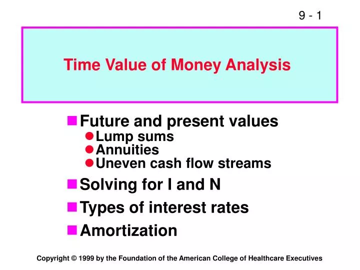
Time Value of Money Analysis. Future and present values Lump sums Annuities Uneven cash flow streams Solving for I and N Types of interest rates Amortization. Time Value -- What is it??. The cost of time -- opportunity cost of money Relationship between asset value and future cash flows

E N D
Time Value of Money Analysis • Future and present values • Lump sums • Annuities • Uneven cash flow streams • Solving for I and N • Types of interest rates • Amortization
Time Value -- What is it?? • The cost of time -- opportunity cost of money • Relationship between asset value and future cash flows • Examples - real estate and GE stock
Time Value -- What is it?? • Relationship between future cash flows and asset value changes • The role of time value analysis • Types of analysis - future value and present value analysis
Terminology of Time Value Analysis • Present value • Future value • Interest rate • Discount rate • Cash flow
Terminology of Time Value Analysis • Time Line • Lump sum • Annuity • Uneven cash flows
Time Lines 1 2 0 3 I% CF0 CF1 CF2 CF3 Tick marks designateends of periods. Time 0 is today (the beginning of Period 1); Time 1 is the end of Period 1 (the beginning of Period 2); and so on.
Time Line Illustration 1 (Lump sum) 1 0 2 5% $100 • What does this time line show?
Time Line Illustration 2 (annuity) 0 1 2 3 10% $100 $100 $100 • What does this time line show?
Time Line Illustration 3 (uneven cash flows) 0 1 2 3 6% -50 100 75 50 • What does this time line show?
What is the FV after 3 years ofa $100 lump sum invested at 10%? 0 1 2 3 10% -$100 FV = ? • Finding future values (moving to the right along the time line) is called compounding. • For now, assume interest is paid annually.
After 1 year: FV1 = PV + INT1 = PV + (PV x I) = PV x (1 + I) = $100 x 1.10 = $110.00. After 2 years: FV2 = FV1 + INT2 = FV1 + (FV1 x I) = FV1 x (1 + I) = PV x (1 + I) x (1 + I) = PV x (1 + I)2 = $100 x (1.10)2 = $121.00.
After 3 years: FV3 = FV2 + I3 = PV x (1 + I)3 = 100 x (1.10)3 = $133.10. In general, FVN = PV x (1 + I)N .
Three Primary Methods to Find FVs • Solve the FV equation using a regular (non-financial) calculator. • Use a financial calculator; that is, one with financial functions. • Use a computer with a spreadsheet program such as Excel, Lotus 1-2-3, or Quattro Pro.
Non-Financial Calculator Solution 0 1 2 3 10% -$100 $133.10 $110.00 $121.00 $100 x 1.10 x 1.10 x 1.10 = $133.10.
Financial Calculator Solution • Financial calculators are pre-programmed to solve the FV equation: FVN = PV x (1 + I)N. • There are four variables in the equation: FV, PV, I and N. If any three are known, the calculator can solve for the fourth (unknown).
Using a calculator to find FV (lump sum): INPUTS 3 10 -100 0 N I/YR PV PMT FV 133.10 OUTPUT Notes: (1) For lump sums, the PMT key is not used. Either clear before the calculation or enter PMT = 0. (2) Set your calculator on P/YR = 1, END.
Types of Annuities Ordinary Annuity 0 1 2 3 I% PMT PMT PMT Annuity Due 0 1 2 3 I% PMT PMT PMT
What is the FV of a 3-year ordinary annuity of $100 invested at 10%? 0 1 2 3 10% $100 $100 $100 110 121 FV = $331
Financial Calculator Solution INPUTS 3 10 0 -100 331.00 N I/YR PV PMT FV OUTPUT Have payments but no lump sum, so enter 0 for present value.
What is the FV if the annuity were an annuity due? • Do ordinary annuity calculation as described before • Multiply result by (1 + interest rate)
What is the PV of $100 duein 3 years if I = 10%? (lump sum) 0 1 2 3 10% $100 PV = ? Finding present values (moving to the left along the time line) is called discounting.
Solve FVN = PV x (1 + I )N for PV: PV = FVN / (1 + I )N. PV = $100 / (1.10)3 = $100(0.7513) = $75.13.
Financial Calculator Solution INPUTS 3 10 0 100 -75.13 N I/YR PV PMT FV OUTPUT Either PV or FV must be negative on most calculators. Here, PV = -75.13. Put in $75.13 today, take out $100 after 3 years.
Opportunity Costs • On the last illustration we needed to apply a discount rate. Where did it come from? • The discount rate is the opportunity cost rate. • It is the rate that could be earned on alternative investments of similar risk. • It does not depend on the source of the investment funds.
What is the PV of this ordinary annuity? 0 1 2 3 10% $100 $100 $100 $90.91 82.64 75.13 $248.68 = PV
INPUTS 3 10 100 0 N I/YR PV PMT FV OUTPUT -248.69 This problem has payments but no lump sum, so enter 0 for future value.
What is the PV if the annuity were an annuity due? 0 1 2 3 10% $100 $100 $100 ? ?
What is the PV if the annuity were an annuity due? • Calculate present value of ordinary annuity as described above • Multiply result by (1 + interest rate) • Annuities due not as common as ordinary annuities
Switch from End to Begin mode on a financial calculator. Repeat the annuity calculations. PV = $273.55. INPUTS 3 10 100 0 -273.55 N I/YR PV PMT FV OUTPUT
Perpetuities • A perpetuity is an annuity that lasts forever. • What is the present value of a perpetuity? PV (Perpetuity) = . PMT I
Uneven Cash Flow Streams: Setup 4 0 1 2 3 10% $100 $300 $300 -$50 $ 90.91 247.93 225.39 -34.15 $530.08 = PV
Uneven Cash Flow Streams:Financial Calculator Solution • Input into “CF” registers: CF0 = 0 CF1 = 100 CF2 = 300 CF3 = 300 CF4 = -50 • Enter I = 10%, then press NPV button to get NPV (PV) = $530.09.
Will the FV of a lump sum be larger or smaller if we compound more often, holding the stated I% constant? Why? LARGER! If compounding is more frequent than once a year--for example, semiannually, quarterly, or daily--interest is earned on interest more often.
0 1 2 3 10% -100 133.10 Annual: FV3 = 100 x (1.10)3 = 133.10. 0 1 2 3 4 5 6 0 1 2 3 5% -100 134.01 Semiannual: FV6 = 100 x (1.05)6 = 134.01.
We will deal with 3 different rates: IStated = stated, or nominal, or quoted, rate per year. IPeriod = periodic rate. EAR = effective annual rate.
IStated is the rate given in contracts. • Often an annual rate. • Compounding periods (M) may be given: • 8% compounded quarterly. • 12% compounded monthly. • IPeriod is the rate per period. • IPeriod = IStated / M. • For 8% compounded quarterly: periodic rate = 2%. • For 12% compounded monthly: periodic rate = 1%.
Effective Annual Rate (EAR) • EAR is the annual rate which causes any PV to grow to the same FV as under intra-year compounding. • What is the EAR for 10%, semiannual compounding? • Consider the FV of $1 invested for one year. FV = $1 x (1.05)2 = $1.1025. • EAR = 10.25%, because this rate would produce the same ending amount ($1.1025) under annual compounding.
The EAR Formula M IStated EAR = 1 + - 1.0 M 2 0.10 = 1 + - 1.0 2 = (1.05)2 - 1.0 = 0.1025 = 10.25%. Or use the EFF% key on a financial calculator.
EAR of 10% at Various Compounding EARAnnual = 10%. EARQ = (1 + 0.10/4)4 - 1.0 = 10.38%. EARM = (1 + 0.10/12)12 - 1.0 = 10.47%. EARD(360) = (1 + 0.10/360)360 - 1.0 = 10.52%.
What’s the value at the end of Year 3of the following CF stream if the stated interest rate is 10%, compounded semiannually? 4 5 0 1 2 3 6 6-month periods 5% $100 $100 $100 • Note that payments occur annually, but compounding occurs semiannually, so we can not use normal annuity valuation techniques.
First Method: Compound Each CF 0 1 2 3 4 5 6 5% $100 $100.00 $100 110.25 121.55 $331.80
Second Method: Treat as an Annuity • Find the EAR for the stated rate: EAR = (1 + ) - 1 = 10.25%. 2 0.10 2 • Then use standard annuity techniques: 3 10.25 0 -100 INPUTS N I/YR PV FV PMT 331.80 OUTPUT
Amortization Construct an amortization schedule for a $1,000, 10% annual rate loan with 3 equal payments.
Step 1: Find the required payments. 0 1 2 3 10% -$1,000 PMT PMT PMT 3 10 -1000 0 402.11 INPUTS N I/YR PV FV PMT OUTPUT
Step 2: Find interest charge for Year 1. INTt = Beginning balance x I. INT1 = $1,000 x 0.10 = $100. Step 3: Find repayment of principal in Year 1. Repmt = PMT - INT = $402.11 - $100 = $302.11.
Step 4: Find ending balance at end of Year 1. End bal = Beg balance - Repayment = $1,000 - $302.11 = $697.89. Repeat these steps for Years 2 and 3 to complete the amortization table.
BEG PRIN END YR BAL PMT INT PMT BAL 1 $1,000$402$100$302$698 2 69840270332366 3 366402373660 TOT $1,206.34$206.34$1,000 Note that annual interestdeclines over time while the principal paymentincreases.
$ 402.11 Interest 302.11 Principal Payments 0 1 2 3 Level payments. Interest declines because outstanding balance declines. Lender earns 10% on loan outstanding, which is falling.