Download
1 / 28
280 likes | 286 Views
Statistics of Visual Binaries and Star Formation History. Oleg Malkov Institute of Astronomy Rus. Acad. Sci. (INASAN) Faculty of Physics, Moscow State University malkov@inasan.ru. Contents. Introduction Initial distributions Evolutionary stages Observational data for comparison

E N D
Statistics of Visual Binaries and Star Formation History Oleg Malkov Institute of Astronomy Rus. Acad. Sci. (INASAN) Faculty of Physics, Moscow State University malkov@inasan.ru MSA-2017
Contents • Introduction • Initial distributions • Evolutionary stages • Observational data for comparison • Results of comparison • Conclusions MSA-2017
Introduction • Most stars formed as part of a binary or multiple systems. • In order to understand the star formation process, it is vital to characterize distributions of physical parameters in the history of the Galaxy. • In the solar neighborhood limit, few hundred parsec of distance, most of the binary systems are visual binaries. • We begin from the assumption that all stars born in a binary system. • Evolutionary stage is calculated as a function of system age and component masses. • Observational selection effects are involved. • Thus, we modeled visual binaries in the solar neighborhood and compare our calculations with observations. MSA-2017
Initial distributions MSA-2017
Spatial distribution • Uniform • Barometric: GALACTIC_DISC_VERTICAL_SCALE_PC = 200 • Barometric: GALACTIC_DISC_VERTICAL_SCALE_PC = • 50 for mass>10, • 10-0.832*log(mass)+2.531 for 1<=mass<=10, • 340 for mass<1, • (Gilmore and Reid 1983, Kroupa 1992, Reed 2000) • No radial gradient MSA-2017
Number of pairs simulated • Sphereradius = 500 pc • Pairs are simulated until their number in a 100-pc-sphere reaches 500,000 • It corresponds to the observed stellar density in the solar vicinity, about 0.12-0.14 stars per cubic pc MSA-2017
Pairing scenarios: masses. 1 • Select (two) fundamental parameters among m1, m2, m1+m2, m2/m1, m1-m2, m1*m2, … • The following scenarios are used • m1, m2 (RP, random pairing) • m1, m2/m1 (PCP, primary constrained pairing) • m1+m2, m2/m1 (SCP, split-core pairing) • m1+m2, m1 (TPP, total and primary pairing) MSA-2017
Pairing scenarios: masses. 2 • Select method of treating low-mass companions (m2<mmin): • Accept (even stars with a planetary companion are considered to be in a binary system) • Reject (the primary star becomes a single star) • Redraw (it is rejected, and a new companion star is drawn) • Method of treating low-mass companions (m2<mmin): Accept MSA-2017
Mass distribution • Masses are distributed according to a power-law function N(m) ~ mα from 0.08 to 100 msun • Salpeter IMF: α=-2.35 • Kroupa IMF: • α=-1.3 for m<0.5 msun • α=-2.3 for m≥0.5 msun • Later: vary slopes and inflection points of Kroupa IMF MSA-2017
Total mass and mass ratio distributions • m1+m2 (strictly speaking, it does not precisely equal protobinary cloud mass): is distributed like masses of individual stars • f(q) ~ qβ, where β = 0, -0.5, +0.5 • Later: add twins (q=1) MSA-2017
Semi-major axis distribution • f(a) ~ aλ, where λ=-1, -1.5, -2 • Lower limit is 10 Rsun, upper limit is 106 Rsun • λ = -1: uniform logarithmic distribution along five orders of magnitude • Later: • lower limit depends on stellar mass, amin=amin(RocheLobe(m)) • upper limit amax=amax(height scale z, mass, eccentricity) MSA-2017
Eccentricity distribution • f(e) = 2e • f(e) = δ(0) • f(e) = 1 MSA-2017
Star formation rate • Constant star formation rate from 0 to DISCAGE = 14 Gyr • Declining star formation rate from 0 to DISCAGE = 14 Gyr: SFR(t)=15e-(t/τ), where τ=7Gyr • Verification: the function produces • current SFR = 3.6 msun/yr, which is correct • integral mass 8*1010msun, which is equal to Galaxy mass MSA-2017
Other parameters • Metallicity: normal Fe/H distribution with mean=-0.1 and dispersion 0.3 • Random distributions for: mean anomaly, sin(inclination), position angle, periastron longitude • Interstellar extinction Av=0 MSA-2017
Evolution MSA-2017
Evolution stage (mass, age) • BD • Pre-MS • MS • RG • WD • NS • BH MSA-2017
Evolution stage (mass, age) MSA-2017
Evolution stage (mass, age) MSA-2017
HR diagram MSA-2017
Observational data for comparison: WDS+CCDM+TDSC binaries with TGAS parallaxes MSA-2017
Selection criteria • Main component belongs to MS • Secondary component is not degenerate • Separation ρ > 1 arcsec • Primary brightness V1 < 10m • Secondary brightness V2 < 11m • Brightness difference (V2-V1) < 4m • Distance d < 500 pc (π > 2 mas) • Altogether 1028 systems MSA-2017
Numbers/distributions for comparison • Number of selected stars • Distributions over V1, V2, V2-V1, ρ”, ρRsun, π“ (χ2 test) • Overall χ2 value, based on distributions of independent, original parameters (V1, V2-V1, ρ”, π“) MSA-2017
An example: TPP (m1+m2, m1), Kroupa IMF,f(a) ~ a-1.5, f(e) = 1 ρ” V2-V1 V1 π" MSA-2017
Results of comparison MSA-2017
Resume. 1 • Results weakly depend on eccentricity distribution. • It is difficult to make conclusions on mass ratio (q) distribution. MSA-2017
Scenario, IMF f(a) ~ aλ MSA-2017
Resume. 2 • PCP (m1, q), RP (m1, m2) and SCP (m1+m2, q) scenarios show a good agreement with observations. • Kroupa IMF is slightly more preferable than Salpeter IMF. • Semi-major axis distributions f(a) ~ aλ, where λ=-1 and -1.5, look very promising, and will be analyzed in detail. Distribution with λ=-2 should be omitted from further consideration. MSA-2017
Acknowledgments • Co-authors • RFFR 15-02-04053 • Audience for your attention MSA-2017