Download
1 / 16
220 likes | 547 Views
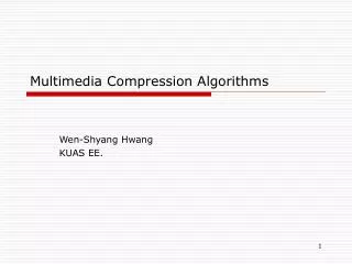
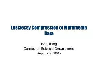
Multimedia Data Compression Part II. Chapter 8 Lossy Compression Algorithms. 1. Li & Drew. Chapter 8 Lossy Compression Algorithms. 8.1 Introduction 8.2 Distortion Measures 8.3 The Rate-Distortion Theory 8.4 Quantization 8.5 Transform Coding 8.6 Wavelet-Based Coding. 8.1 Introduction.

E N D
Multimedia Data Compression Part II Chapter 8 Lossy Compression Algorithms 1 Li & Drew
Chapter 8Lossy Compression Algorithms 8.1 Introduction 8.2 Distortion Measures 8.3 The Rate-Distortion Theory 8.4 Quantization 8.5 Transform Coding 8.6 Wavelet-Based Coding
8.1 Introduction • Lossless compression algorithms do not deliver compression ratios that are high enough. Hence, most multimedia compression algorithms are lossy. • What is lossy compression? – The compressed data is not the same as the original data, but a close approximation of the original image perceptually. – Yields a much higher compression ratio than that of lossless compression. 3 Li & Drew
8.2 Distortion Measures • A distortion measure is a mathematical quantity that specifies how close an approximation is to its original, using some distortion criteria. • The three most commonly used distortion measures in image compression are: – mean square error (MSE) σ2, (8.1) where xn, yn, and N are the input data sequence, reconstructed data sequence, and length of the data sequence respectively. – signal to noise ratio (SNR), in decibel units (dB), (8.2) where is the average square value of the original data sequence and is the MSE. – peak signal to noise ratio (PSNR), (8.3) 4 Li & Drew
8.3 The Rate-Distortion Theory • Provides a framework for the study of tradeoffs between Rate and Distortion. • Rate is: the average number of bits required to represent each source symbol. • From figure: the minimum possible rate at D=0, no loss. The distortion corresponding to a rate R(D)=0 is the maximum amount of distortion incurred when “nothing” is coded. 5 Li & Drew
8.4 Quantization • Reduce the number of distinct output values to a much smaller set. • Main source of the “loss” in lossy compression. • Three different forms of quantization. – Uniform: midrise and midtread quantizers. – Nonuniform: companded quantizer. – Vector Quantization. 6 Li & Drew
8.5 Transform Coding • The rationale behind transform coding: If Y is the result of a linear transform T of the input vector X in such a way that the components of Y are much less correlated, then Y can be coded more efficiently than X. • If most information is accurately described by the first few components of a transformed vector, then the remaining components can be coarsely quantized, or even set to zero, with little signal distortion. • Transformation to the frequency domain via Discrete Cosine Transform (DCT), Wavelet Transform (WT) and Fourier Transform (FT). 7 Li & Drew
Spatial Frequency and DCT • Spatial frequency indicates how many times pixel values change across an image block. • The DCT formalizes this notion with a measure of how much the image contents change in correspondence to the number of cycles of a cosine wave per block. • The role of the DCT is to decompose the original signal into its DC and AC components; the role of the IDCT is to reconstruct (re-compose) the signal. 8 Li & Drew
Fig. 8.9: Graphical Illustration of 8 × 8 2D DCT basis. 9 Li & Drew
8.6 Wavelet-Based Coding • The objective of the wavelet transform is to decompose the input signal into components that are easier to deal with, have special interpretations, or have some components that can be thresholded away, for compression purposes. • We want to be able to at least approximately reconstruct the original signal given these components. • The basis functions of the wavelet transform are localized in both time and frequency. • There are two types of wavelet transforms: the continuous wavelet transform (CWT) and the discrete wavelet transform (DWT). 10 Li & Drew
Li & Drew Wavelet Transform Example • Suppose we are given the following input sequence. • {xn,i} = {10, 13, 25, 26, 29, 21, 7, 15} • Consider the transform that replaces the original sequence with its pairwise averagexn−1,i and differencedn−1,i defined as follows: • The averages and differences are applied only on consecutive pairs of input sequences whose first element has an even index. Therefore, the number of elements in each set {xn−1,i} and {dn−1,i} is exactly half of the number of elements in the original sequence.
Li & Drew • • Form a new sequence having length equal to that of the original sequence by concatenating the two sequences {xn−1,i} and {dn−1,i}. The resulting sequence is • {xn−1,i, dn−1,i} = {11.5, 25.5, 25, 11,−1.5,−0.5, 4,−4} • • This sequence has exactly the same number of elements as the input sequence — the transform did not increase the amount of data. • • Since the first half of the above sequence contain averages from the original sequence, we can view it as a coarser approximation to the original signal. The second half of this sequence can be viewed as the details or approximation errors of the first half.
Li & Drew • • It is easily verified that the original sequence can be reconstructed from the transformed sequence using the relations • xn, 2i= xn−1, i + dn−1, i • xn, 2i+1 = xn−1, i− dn−1, i • • This transform is the discrete Haar wavelet transform. • Fig. 8.12: Haar Transform: (a) scaling function, (b) wavelet function.
2D Wavelet Transform • • For an N by N input image, the two-dimensional DWT proceeds as follows: – Convolve each row of the image with low-pas and high-pass filters, discard the odd numbered columns of the resulting arrays, and concatenate them to form a transformed row. – After all rows have been transformed, convolve each column of the result with low-pass and high-pass filters. Again discard the odd numbered rows and concatenate the result. • • After the above two steps, one stage of the DWT is complete. The transformed image now contains four subbands LL, HL, LH, and HH, standing for low-low, high-low, etc. • • The LL subband can be further decomposed to yield yet another level of decomposition. This process can be continued until the desired number of decomposition levels is reached. 14 Li & Drew
Fig. 8.19: The two-dimensional discrete wavelet transform (a) One level transform, (b) two level transform. 15 Li & Drew
2D Wavelet Transform Example 16 Li & Drew