Download
1 / 48
480 likes | 793 Views
Topic 4 Data Mining. Resources: See References slide. Knowledge discovery and data mining. “ Knowledge discovery in databases is the non-trivial process of identifying valid, novel, potentially useful, and ultimately understandable patterns in data.”

E N D
Topic 4Data Mining Resources: See References slide
Knowledge discovery and data mining “Knowledge discovery in databases is the non-trivial process of identifying valid, novel, potentially useful, and ultimately understandable patterns in data.” “Data mining is a step in the KDD process consisting of applying data analysis and discovery algorithms that, under acceptable computational efficiency limitations, produce a particular enumeration of patterns over the data.” Fayyad et al., 1996.
What is data mining? • An important component of knowledge discovery in databases (KDD) • Data preparation • Data selection • Data cleaning • Incorporating prior knowledge • Data mining • Result interpretation increasing sophistication Data mining SQL OLAP co-occurrence, correlation, causation Select avg(salary) From Employees Group by dept; aggregates in multiple dimensions Adapted from Luis Gravano’s Advanced Databases course
Other fun quotes • Why we need data mining • "Drowning in data yet starving for knowledge", anonymous • "Computers have promised us a fountain of wisdom but delivered a flood of data", W. J. Frawley, G.Piatetsky-Shapiro, and C. J. Matheus • “Where is the wisdom we have lost in knowledge? Where is the knowledge we have lost in information?”, T. S. Eliot • What data mining is not • Data mining, noun: "Torturing data until it confesses ... and if you torture it enough, it will confess to anything", Jeff Jonas, IBM • "An unethical econometric practice of massaging and manipulating the data to obtain the desired results", W.S. Brown “Introducing Econometrics” From http://www.cs.ccsu.edu/~markov/ccsu_courses/DataMining-1.html
Is data mining a discipline? • Data mining vs. statistics • Statistics is largely quantitative, DM is qualitative • DM focuses on exploratory analysis, not on hypothesis testing • A large component of DM is cleaning / preprocessing • Data mining vs. machine learning • DM is significantly influenced by ML, but • Often focuses on incomplete / dirty real world data • Not typically concerned with learning a general model from the data • Efficiency and scalability are important • Data may be updated • Domain knowledge may be given in the form of integrity constraints • Yes, data mining is a discipline in which statistics, databases, machine learning, data visualization, …. come together
Types of data mining analysis • Association rule mining • e.g., 72% of customers who bought cookies also bought milk • focus of parts 1 and 2 of today’s lecture • Finding sequential / temporal patterns • e.g., find the set of genes that are differentially expressed, and whose expression precedes the onset of a disease • Classification • e.g., Is a new customer applying for a loan a good investment or not? if STATUS = married and INCOME > 50K and HOUSE_OWNER = yes then INVESTMENT_TYPE = good -- or is it? • Clustering • Similar to classification, but classes are not known ahead of time • will see an example in part 3 of today’s lecture
Roadmap • Introduction → Association rule mining • Mining generalized association rules • Subspace clustering
Association rule mining • Proposed by Agrawal, Imielinski and Swami in SIGMOD 1993 • The now-classic Apriori algorithm by Agrawal and Srikant was published in VLDB 1994, received the 10-year best paper award at VLDB 2004 • Initially used for market basket data analysis, but has many other applications • Answers two related questions • Which items are often purchased together? • frequent itemsets, e.g., Milk, Cookies • have an associated support • Which items will likely be purchased, based on other purchased items? • association rules, e.g., Diapers => Beer • meaning: if diapers are bought in a transaction, beer is also likely bought in the same transaction. • each association rule is derived from two frequent itemsets • have an associated support and condifence
The model: market-basket data • I = {i1, i2, …, im}: the set of all available items • e.g., a product catalog of a store • Transaction t: a set of items purchased together, tI • has a transaction id (TID) t1: {bread, cheese, milk} t2: {apple, eggs, salt, yogurt} t3: {biscuit, cheese, eggs, milk} • Transaction Database T: a set of transactions {t1, t2, …, tn} • What is not represented by this model?
Text documents as transactions • Each document is a bag of words doc1: Student, Teach, School doc2: Student, School doc3: Teach, School, City, Game doc4: Baseball, Basketball doc5: Basketball, Player, Spectator doc6: Baseball, Coach, Game, Team doc7: Basketball, Team, City, Game
Itemsets • X I is an itemset • X = {milk, bread, cereal} is an itemset • X is a 3-itemset (a k-itemset with k=3) • X has support supp if supp% of transactions contain X • A transaction t contains an itemset X if Xt • t is said to give support to X • A user specifies a support threshold minSupp • Itemsets with support > minSupp are frequent itemsets • Example
Association Rules • An association rule is an implication of the form X Y, where X, Y I, and X Y = • {milk, bread} {cereal} is an association rule • meaning: “A customer who purchased X is also likely to have purchased Y in the same transaction” • we are interested in rules with a single item in Y • can we represent {milk, bread} -> {cereal, cheese}? • The rule X Y holds with supportsupp in T if supp % of transactionscontain X Y • supp ≈ Pr(X Y) • The rule holds in T with confidence conf if conf % of transactions that contain X also contain Y • conf≈ Pr(Y | X) • conf (X Y) = supp (X U Y) / supp (X)
Association Rule Mining • Goal: find all association rules that satisfy the user-specified minimum support and minimum confidence • Algorithm outline • Step 1: find all frequent itemsets • Step 2: find association rules • Take 1: naïve algorithm for frequent itemset mining • Enumerate all subsets of I, check their support in T • What is the complexity? • Any obvious optimizations?
Downward Closure • Recall: a frequent itemset has support ≥minSupp • Key idea: Use the downward closure property • all subsets of a frequent itemset are themselves frequent • conversely: if an itemset contains any infrequent itemsets as subsets, it cannot be frequent (we know this apriori) • Is an itemset necessarily frequent if all its subsets are frequent? • No! supp(X U Y) < supp(X) + supp(Y) ABC ABD BCD ACD AB AC BC BD CD AD A B C D
The Apriori Algorithm Algorithm Apriori(T) F1 = {frequent 1-itemsets}; for (k = 2; Fk-1; k++) do Ck candidate-gen(Fk-1); for each transaction tTdo for each candidate cCkdo ifc is contained in tthen c.count++; end end Fk {cCk | c.count/nminsup} end return FkFk;
Apriori candidate generation • The candidate-gen function takes Fk-1 and returns a superset(called the candidates)of the set of all frequent k-itemsets.It has two steps • Join: generate all possible candidate itemsets Ck of length k • Prune: remove those candidates in Ck that have infrequent subsets • Which subsets do we check?
The Candidate-gen Function Assume a lexicographic ordering of the items Join Insert into Ck Select p.item1, p.item2, …, p.itemk-1, q.itemk-1 From Ck-1 p, Ck-1 q Where p.item1 = q.item1 And p.item2 = q.item2 And …. And p.itemk-1 < q.itemk-1Why not p.itemk-1 ≠ q.itemk-1? Prune for each c in Ck do for each (k-1) subset s of c do if (s not in Ck-1) then delete c from Ck
Generating Association Rules • For each frequent k-itemset X • for each k-1-itemset AX • let B = X - A • compute conf (A B) = supp (X) / supp (A) • if conf(A B) > minConf then A B is an association rule • Example • How are association rules different from functional dependencies in databases?
Performance of Apriori • The possible number of frequent itemsets is exponential, O(2m), where m = |I| • The Apriori algorithm exploits sparseness and locality of data • Still, it may produce a large number of rules: thousands, tens of thousands, …. • So, thresholds should be set carefully– What are some good heuristics? • Let’s take another look at the algorithm
The Apriori Algorithm Algorithm Apriori(T) F1 = {frequent 1-itemsets}; for (k = 2; Fk-1; k++) do Ck candidate-gen(Fk-1); for each transaction tTdo // a full scan of the database for each k! for each candidate cCkdo ifc is contained in tthen c.count++; end end Fk {cCk | c.count/nminsup} end return FkFk;
The AprioriTid Algorithm Algorithm AprioriTid(T) F1 = {frequent 1-itemsets}; T1 = T for (k = 2; Fk-1; k++) do Ck candidate-gen(Fk-1); Tk = {} for each transaction tTk-1do Ckt = {itemsets in Ck to which t gives support} for each candidate cCktdo c.count++; end Tk = Tk U <t.TID, Ckt > end Fk {cCk | c.count/nminsup} end return FkFk;
Apriori vs. AprioriTid • Any guesses as to the relative performance? • the goal is to avoid scanning the database T • so, we are computing and carrying around a redundant data structure that contains a sub-set of T, in conveniently pre-processed form • When does this NOT help performance? • for small k? for large k?
So, why the 10-year best paper award? • Why is this such a big deal? • A fairly simple model • A fairly simple bottom-up algorithm • A fairly obvious performance optimization • No pretty optimality proof • But this is only simple in hindsight! Plus…. • The algorithm works well in practice • Many real applications • Many possible useful extensions, will look some in the remainder of today’s lecture
Roadmap • Introduction • Association rule mining • Generalized association rule mining • Subspace clustering
Generalized Association Rules clothes footwear outerwear shirt shoes boots minSupp = 30% minConf = 60% pants jacket
Generalized Association Rules clothes (4) footwear (4) outerwear (3) shirt (1) shoes (3) boots (2) pants (1) Observations (X’ denotes an ancestor of X) supp (footwear) ≠ supp (shoes) + supp (boots) supp(X U Y) > minSupp what about supp (X’ U Y) and supp (X’ U Y’)? 3. supp (X Y) > minSupp, conf (X Y) > minConf what about supp, conf of X Y’, X’ Y, X’ Y’? jacket (2)
Interesting Rules • Fact: A1: milk -> cereal (8% supp, 70% conf) • Fact: about ¼ of sales of milk are for skim milk • What is the expected strength of A2: skim milk -> cereal ? • If (2% support, 70% confidence), then A2 is redundant: less general than A1, but support and confidence are as expected • Interesting rules have confidence, or support, R times higher than expected value • the interest threshold is specified by the user • More details in [Srikant and Agrawal, VLDB 1995].
Algorithm Outline • Find all frequent generalized itemsets (support > minSupp) – we focus on this step • Use frequent itemsets to generate association rules (confidence > minConf) • Prune all uninteresting rules Can we modify Apriori to find generalized itemsets?
Apriori clothes footwear • Modify T: include ancestors of each item into each transaction, remove duplicates; call this T’ • Call Apriori (T’) outwear shirt shoes boots pants jacket
Apriori – any problems? • Rules that contain an item and its ancestor: are these meaningful? • shoes -> footwear • footwear -> shoes • footwear, outerwear -> shoes • footwear, shoes -> outerwear • Do we always care to have all ancestors? • No, only if the ancestor is in at itemset being considered in the current iteration • But now we have to modify transactions as we go, not in a single pre-processing step • What’s a good way to transform T -> T’? • Pre-compute transitive closure • Apriori Cumulate contains these optimizations
AprioriCumulate Algorithm AprioriCumulate(T) I* = transitiveClosure(I); // how do we represent this? F1 = {frequent 1-itemsets}; for (k = 2; Fk-1; k++) do Ck candidate-gen(Fk-1); if (k = 2) then delete all c in Ck that consist of an item and its ancestor; I*k = I* without ancestors that do not appear in Ck for each transaction tTdo add all ancestors of items in t that appear in I*k to t for each candidate cCkdo ifc is contained in tthen c.count++; end end Fk {cCk | c.count/nminsup} end return FkFk;
Recap • An extension of frequent itemset mining • Realistic application scenario • Similar to Apriori, but with some new semantic considerations • Some rules are more interesting than others • New optimizations are possible • Apriori Cumulate • other algorithms have been proposed: Apriori Stratify, Estimate, EstMerge,see paper
Roadmap • Introduction • Association rule mining • Generalized association rule mining • Subspace clustering
Clustering of high-dimensional data • Relational data with d numerical attributes • e.g., profiles of people in a dating site: age, height income, net worth, number of children, … • e.g., expression levels of genes in a microarray experiments, under a variety of conditions • Desiderata • Interpret data by organizing it into groups, e.g., high income, education levels, net worth often co-occur • Number of groups not known in advance • Groups need to be described to be interpretable • Why is this difficult?
The curse of dimensionality The problem caused by the exponential increase in volume as dimensions are added to a mathematical space. Has a direct effect on distance functions – the minimum and maximum occurring Distances become indiscernible as dimensionality increases Parsons et al., SIGKDD Explorations 6(1), 2006
Dimensionality Reduction • Feature transformation: summarize a dataset in fewer dimensions by combining original dimensions • Useful in discovering latent structure in datasets • Less effective when there many irrelevant attributes that hide the clusters in a sea of noise • Feature selection: select only the most relevant dimensions, project, cluster in reduced space • e.g, Principal Component Analysis (PCA) • But what if clusters exist in different subspaces?
Subspace clustering Parsons et al., SIGKDD Explorations 6(1), 2006
What is subspace clustering? • Identifies clusters in multiple, possibly overlapping, sub-sets of dimensions • Dimensionality reduction per cluster • A cluster described by a combination of dimensions and value ranges, e.g., “age 20-25” and “edu = BS” and “income 25K-50K” • Two main approaches • Top-down: start with full dimensionality and refine • Bottom-up: start with dense units in 1D, merge them to find higher-dimensional clusters
Salary (10,000) 7 6 4 3 2 1 age 20 30 40 50 60 The CLIQUE Algorithm • Identify subspaces that contain clusters • Identify clusters • Generate minimal cluster descriptions (25 < age < 45 AND 3K < salary < 7K) OR (35 < age < 50 AND 2K < salary < 6K)
CLIQUE: Preliminaries • Definitions • A = {A1, …, Ad} is a set of bounded totally ordered domains • S = A1 x … Ad is a d-dimensional numerical space • Input V = {p1, …, pm} is a set of d-dimensional points, each of the form {v1, …, vd} • A subspace of S is a projection onto a subset of the attributes A’ • Units and density • A unit u = {(low1, high1), …, (lowd, highd)}, defined in A or in A’, is a rectangular intersection of intervals in each dimension • A unit contains a point p if lowi< vi < highi for each i • A unit is denseif it contains sufficiently many points
CLIQUE: Preliminaries (2) • Clusters • A cluster is a maximal set of connected dense units • These are usually defined k-dimensional subspaces, hence, subspace clustering • Goal: find clusters, generate cluster descriptions • Inputs: V, density threshold , number of intervals per dimension (equal for all dimensions!)
age: 18-25 age: 26-30 income: 101-125K income 126-150K age: 31-35 age: 36-40 density > 1 income: 76-100K income: 50-75K 43
age: 31-35 age: 36-40 income: 101-150K age: 18-30 Income: 50-75K income: 76-100K age: 18-30 age: 36-40 density > 1 income: 50-75K income: 101-150K 44
The CLIQUE Algorithm • Apriori-style • Uses downward closure: all projections of a dense k-dimensional unit are dense • Build grid: split up each dimension into intervals, count number of points per interval • Merge: concatenate consecutive dense 1-d units • While dense units are found, iteratively increase k Join: create k-dimensional candidates from (k-1)-dimensional dense units Insert into Ck Select u1.[low1, high1), …, u1.[lowk-1, highk-1), u2.[lowk-1, highk-1) From Dk-1 u1, Dk-1 u2 Where u1.attr1 = u2.attr1 And u1.low1 = u2.low1 And u1.high1 = u2.high1 And u1.attr2 = u2.attr2 And u1.low2 = u2.low2 And u1.high2 = u2.high2 And …. And u1.attrk-1 < u2.attrk-1 Prune: remove k-dimensional candidates that don’t have sufficient density (same as in Apriori)
Taxonomy of Subspace Clustering Algorithms Parsons et al., SIGKDD Explorations 6(1), 2006
Recap • Knowledge Discovery and Data Mining • Association rule mining • From frequent itemsets to association rules • Optimize frequent itemset mining using downward closure • Apriori and AprioriTid algorithms • Generalized association rule mining • Items form a taxonomy • Interesting rules • The Cumulate algorithm • Subspace clustering • Beyond categorical (transaction data) • CLIQUE: a density-based clustering algorithm that uses support
References • Fast Algorithms for Mining Association Rules in Large Databases. Rakesh Agrawal and Ramakrishnan Srikant. VLDB 1994. • Mining Generalized Association Rules. Ramakrishnan Srikant and Rakesh Agrawal, VLDB 1995. • Automatic Subspace Clustering of High Dimensional Data for Data Mining Applications. Rakesh Agrawal, Johannes Gehrke, Dimitrios Gunopulos, and Prabhakar Raghavan, SIGMOD 1998.