Download
1 / 38
570 likes | 2.04k Views
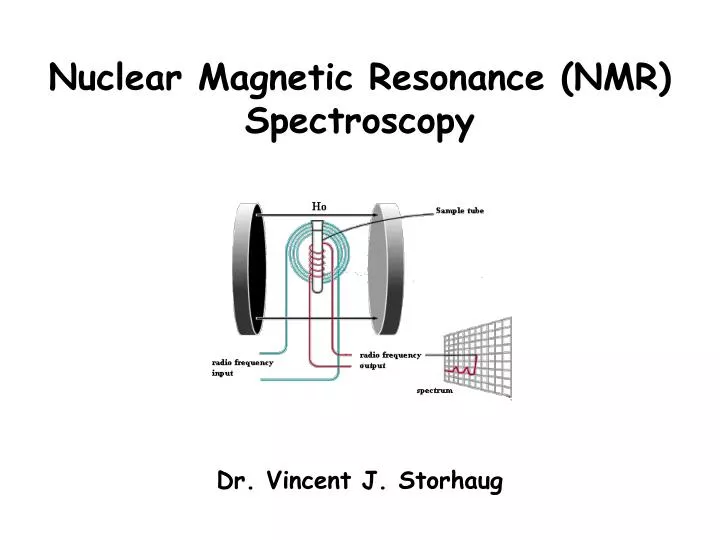
Nuclear Magnetic Resonance (NMR) Spectroscopy. Dr. Vincent J. Storhaug. NMR Spectroscopy. NMR spectroscopy is a form of absorption spectrometry.

E N D
Nuclear Magnetic Resonance (NMR) Spectroscopy Dr. Vincent J. Storhaug
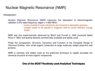
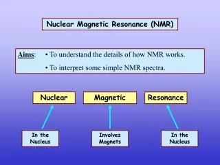
NMRSpectroscopy NMR spectroscopy is a form of absorption spectrometry. Most absorption techniques (e.g. – Ultraviolet-Visible and Infrared) involve the electrons… in the case of NMR, it is the nucleus of the atom which determines the response. An applied (magnetic) field is necessary to “develop” the energy states (produce a separation of the energy states) necessary for the absorption to occur.
Development of Energy States of Nuclei in an Applied Magnetic Field Spin ½ Nucleus = “Bar Magnet”
Development of Energy States of Nuclei in an Applied Magnetic Field Spin ½ Nucleus = “Bar Magnet”
Applied Magnetic Field Bo Populations of the Energy States of Hydrogen Nuclei (Spin ½ Nuclei) in a Magnetic Field Ea Without an applied magnetic field, there is no division of energy states to discuss.
Development of Energy States of Nuclei in an Applied Magnetic Field The nuclei have a property of “spin”, characterized by: p angular momentum quantized in units of h/(2π) I spin quantum number will be in integer or half-integer values This angular momentum is directly related to the magnetic dipole moment, μ, by γ magnetogyric ratio, dependent on the type of nucleus
Development of Energy States of Nuclei in an Applied Magnetic Field There will be 2I+1 discrete energy states, as indicated by: ●●● I I-1 I-2 -I This value is called the magnetic quantum state, mI. The simplest situation, therefore is a system of two energy states, i.e. – I = ½. The value of I for 1H, 13C, 19F, and 31P is ½, so we have: ½ -½
Magnetic Properties of the Four Most Commonly Observed Nuclei Magnetogyric Ratio (radian T-1 s-1) Relative Sensitivity Absorption Frequency (MHz) Nucleus 1H 13C 19F 31P 2.6752 x 10⁸ 6.7283 x 10⁷ 2.5181 x 10⁸ 1.0841 x 10⁸ 1.00 0.016 0.83 0.066 400 100.6 376.5 162.1 All of these nuclei have spin I = ½! http://www.chem.tamu.edu/services/NMR/periodic/index.shtml
In general, the potential energy, E, of a given energy state/orientation is related to the magnetic quantum number by: Applied Magnetic Field Bo Development of Energy States of Nuclei in an Applied Magnetic Field Potential energy, E, and the energy difference between two given states: 0
Transition of Nucleus from One Energy State to Another Planck relationship, between ΔE and an applied radio frequency, ν0 is:
Relationship Between Resonance Frequency and the Applied Field Strength
Boltzmann Distribution of Nuclei Among the Energy Levels Nj the number or nuclei occupying the higher energy state N0 the number or nuclei occupying the lower (ground) energy state Since (for “NMR active” nuclei) when you apply a magnetic field, Bo , a nonzero difference between the energy states develops, ΔE, then we know that Njwill always be smaller than N0.
Boltzmann Distribution of Nuclei Among the Energy Levels Experimentally, we can do only two things in order to increase the difference in populations of the ground and excited states: 1. We can increase the strength of the applied field, B0. 2. We can decrease the absolute temperature, T.
Example Calculation of the Distribution of Nuclei Among the Energy Levels 1H NMR, calculate the ratio Nj/N0, for an NMR system where the magnet has a field of 4.69 T, and the temperature is 20 ºC. i.e. – The populations differ by less than 0.004%!
Basics of Fourier Transform NMR: Relying on Nuclear Precession
Continuous Wave (CW) NMR B0 B0 ω0 ω Absorption* μ μZ μZ μ θ θ Emission ω ω0 m=+1/2 m=-1/2 *Circularly Polarized Radiation μZ magnetic field vector (magnetic vector from the rotating frame of reference) μ spin axis of the nucleus θ angle between the magnetic field vector and the spin axis of the particle
Continuous Wave (CW) NMR • Low magnetic field strength needed (advantage AND disadvantage) • Low sensitivity, and limited to a single sweep of the spectral window • (If you have a small amount of material, you are simply out of luck) • Low resolution (1 Hz linewidth – FWHM - is considered great resolution for CW) • Limited mostly to 1H NMR ONLY. 13C NMR not possible due to decreased sensitivity • (and single sweep) • No computer is necessary, direct plotting of spectrum, but also no way to digitally • save spectrum.
Basics of Fourier Transform NMR: Relying on Nuclear Precession where ω0 is the angular velocity of the precession, in radians/second Experimentally, we need to convert this angular velocity to its corresponding frequency in the electromagnetic spectrum: where υ0 is now in millions of rotations per second units, or commonly, Megahertz (MHz). υ0 is referred to as the Larmor Frequency.
z z y y x x The Fourier Transform Pulsed NMR Technique M0 B0 B0 Laboratory (Static) Frame of Reference Rotating Frame of Reference
“Where the Quantum Explanation Ends, and the Classical One Takes Over”
Basics of Fourier Transform NMR: Relying on Nuclear Precession z Rotating Frame of Reference M0 y x B0
The Fourier Transform Pulsed NMR Technique time Delay Pulse Delay Acquisition time
z z y y x x The Fourier Transform Pulsed NMR Technique(Rotating Frame of Reference) time 90º M0 RF M0 B1 B0 B0
z z y y x x The Fourier Transform Pulsed NMR Technique(Rotating Frame of Reference) α RF M0 Mz My B1 B1 B0 B0 α angle of rotation in radians γ magnetogyric ratio (radians T-1 s-1) B1 induced magnetic field (T) τ pulse width (s)
z y x The Fourier Transform Pulsed NMR Technique(Rotating Frame of Reference) time M0 B0
z z z z y y y y x x x x The Fourier Transform Pulsed NMR Technique(Rotating Frame of Reference) 0 time M0 M0 M0 M0
Basics of Fourier Transform NMR: Measuring the Precession Frequency
Relaxation Process in NMR Spin-Lattice Relaxation, T1 The absorbed energy is lost through vibrational and rotational motion to the magnetic components of the “lattice” of the sample. Problem: The temperature of the sample can rise over time. Spin-Lattice relaxation processes cause an exponential decay of the excited state population. The more viscous a sample is, or the more restricted the motion of a molecule is, the larger the T1. Spin-Lattice relaxation is the slower of the relaxation processes. Spin-Spin Relaxation, T2 Several processes are “lumped” under this term, but one of the predominant techniques is spin diffusion, a process requiring neighboring nuclei to have the same precession rates, but different magnetic quantum numbers. Another cause is a disruption in the homogeneity of the magnetic field through the sample caused by the sample itself. (e.g. – formation of dimers, trimers, etc. that change the relaxation rates of nuclei.) Spin-Lattice relaxation is the faster of the relaxation processes. Thus, T2 is the primary influence on line broadening in the spectrum.
z z z z y y y y x x x x Spin-Spin Relaxation, T2 Mxy time z y x time
z z z z z z z z y y y y y y y y x x x x x x x x Longitudinal Spin-Lattice Relaxation, T1 Mxy time Mz My
Longitudinal Spin-Lattice Relaxation, T1 The time constant, T1,describes how MZ returns to its equilibrium value. The equation governing this behavior as a function of the time t after its displacement is: T1 is therefore defined as the time required to change the Z component of magnetization by a factor of e. If the net magnetization is placed along the “-Z” axis (i.e. – pw = 180º), it will gradually return to its equilibrium position along the “+Z” axis at a rate governed by T1. The equation governing this behavior as a function of the time t after its displacement is:
Relaxation of Mxy During Fourier Transform NMR Responses Due to T1 AND T2
Signal to Noise Improvement With “digital” summations of FIDs (or rather, transients), where n is the total number of scans acquired.
Signal to Noise Improvement: Practical Considerations • Running a 13C NMR spectrum. • Not limited so much in the amount of sample, but by the solubility of the compound in the available solvent (deuterated CDCl3) • Ran the sample for 4 hours, and it looks like: In order to increase the S/N by a factor of 2, this would need to run for 16 hours. In order to increase the S/N by a factor of 4, this would need to run for 64 hours (almost 3 days).
CW vs FT NMR Continuous Wave Fourier Transform • Samples are run “neat” • Less expensive, no deuterated • solvents are necessary • Larger quantities of sample are • needed (gram) • Limited primarily to 1H NMR (dedicated) • Slow acquisition, have to sweep the • frequencies • Signal to Noise limited in what can be • seen in a single sweep • Samples are run diluted • More expensive, MOST of the sample • actually being a deuterated solvent • Very small quantities (<< mg) are • possible • Interchangeable probes, multiple nuclei. • All frequencies are measured in a rapid scan • (milliseconds) • Theoretically, the Signal to Noise is limited • only by the time available to acquire the • spectrum