Download
1 / 17
170 likes | 330 Views
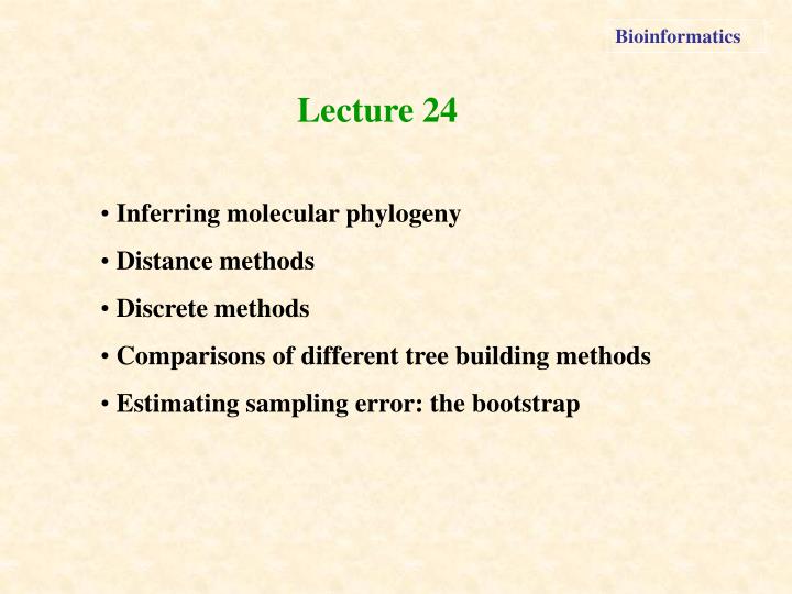
Bioinformatics. Lecture 24. Inferring molecular phylogeny Distance methods Discrete methods Comparisons of different tree building methods Estimating sampling error: the bootstrap. Inferring molecular phylogeny.

E N D
Bioinformatics Lecture 24 • Inferring molecular phylogeny • Distance methods • Discrete methods • Comparisons of different tree building methods • Estimating sampling error: the bootstrap
Inferring molecular phylogeny • The objective of molecular phylogenetics is to convert sequences information (DNA, RNA, proteins) into an evolutionary tree for this sequences. • Ever growing number of tree building methods can very roughly be split into two approaches. • Distance methods versus discrete characters methods. • Clustering methods versus search methods. • These methods will be considered during the lecture.
Distance methods • The simplest distance method based on assumption of constant substitution rates and approximately equal length of neighboring branches called UPGMA (Unweighted Pair Group Method with Arithmetic Mean). • A distance matrix, representing distances between all possible pairs of sequences used for the phylogenetic reconstruction must be built as a first step. • The UPGMA starts from calculating branch length
A C 2 1 4 2 1 B D Distance methods: an idealised case A. Sequences Sequence A ACGCGTTGGGCGATGGCAAC Sequence B ACGCGTTGGGCGACGGTAAT Sequence C ACGCATTGAATGATGATAAT Sequence B ACACATTGAGTGATAATAAT B. Distances between sequences nAB 3 nAC 7 nAD 8 nBC 6 nBD 7 nCD 3 C. Distance table D. The assumed unrooted tree
3.5 3.5 3.5 A A A D D D C C 4.75 4.75 B d(AB)C 2 6.33 d(ADC)B) 2 B C D B C B A 14 11 7 AD 13.5 9.5 ADC 12.67 B - 11 13 B - 11 C - - 8 dAD 2 Values for these tables are calculated from the data presented in the initial table (AD)B = (AB + DB)/2 (ADC)B = (AB + DB + CB)/3 (AD)C = (AC + DC)/2 Diagram illustrating the stepwise construction of a phylogenetic tree for four OTUs according to unweighted pair group method with arithmetic mean (UPGMA). The resulting tree is ultrametric. Methods used: distance and clustering.
Neighbours-joining tree construction. Methods: distance and clustering. H – Human C – Chimpanzee G – Gorilla O – Orangutan R – Rhesus monkey * Number of nucleotide substitutions per 100 sites between OTUs.
Neighbours-relation scores obtained from the distance matrix (see previous slide) Calculation of the total scores: (dHG + dCO) – min score each pair (HG) and (CO) is assigned score of 1; other pairs score 0. As a result the scores are obtained, which are shown in the table. (OR) has the highest total score.
Treating (OR), which has the highest total score, as a separate single OUT, the following table can be calculated. OTU H C G C 1.45 G 1.51 1.57 (OR) 5.25 5.25 5.22 As only 4 OTUs are left, it is easy to see that dHC + dG(OR) = 6.67 < < dHG + dC(OR) = 6.76 < < dH(OR) + DCG = 6.82 Therefore, H and C are chosen as one pair of neighbours G and (OR) as the other. Building Neighbours-Joining (NJ) tree
Site Sequence 1 2 3 4 5 6 7 8 9 1 A A G A G T G C A 2 A G C C G T G C G 3 A G A T A T C C A 4 A G A G A T C C G Inf. sites * * * Maximum parsimonyMethods: discrete characters and search/optimisationInformative sites (*) in four compared sequences, used for phylogenetic reconstruction.
Three possible unrooted trees (I, II and III) for four DNA sequences (1, 2, 3, 4) that have been used to choose the most parsimonious tree.
Comparison of different tree-building methods • Efficiency (how fast is the method?), • Power (how much data does the method need to produce reasonable result?) • Consistency (will it converge on the right answer given enough data?) • Robustness (will minor violations of the method’s assumptions result in poor estimates of phylogeny?) • Falsibility (will the method tell when its assumption violated, in order to avoid using this method)
PARSIMONY UPGMA Performance of UPGMA and parsimony methods The success rate is the percentage of times that the correct tree was recovered in that region of the parameter space. White area in the left top of the both diagram, where non of the methods performs well
MEGA3: Sequence Data Explorer Variable sites Parsimonious sites Sequences continue
Minimum evolution (ME) Neighbor- joining (NJ) Maximum Parsimony (MP) UPGMA MEGA 3: phylogenetic trees
NJ ME MP UPGMA Bootstrapping