Download
1 / 38
380 likes | 388 Views
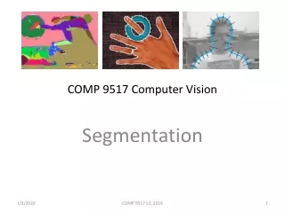
COMP 9517 Computer Vision. Texture. Why texture?. Texture is another feature that help image segmentation and classification Texture provides information about the spatial arrangement of the colours or intensities in an image spatial distribution beside colour/intensity level distribution

E N D
COMP 9517 Computer Vision Texture COMP 9517 S2, 2009
Why texture? • Texture is another feature that help image segmentation and classification • Texture provides information about the spatial arrangement of the colours or intensities in an image • spatial distribution beside colour/intensity level distribution • Texture descriptor provides measures of properties such as smoothness, coarseness, and regularity COMP 9517 S2, 2009
Texture, texels and statistics • It is usually difficult to describe the irregular spatial arrangements • There is some quality of the image that would make on argue that there is a noticeable arrangement in each image • Properties as playing an important role in describing texture: uniformity, density, coarseness, roughness, regularity, linearity, directionality, direction, frequency, and phase. COMP 9517 S2, 2009
Texture, texels and statistics • Structural approach: • A set of primitive texels in some regular or repeated relationship • Statistical approach: • A quantitative measure of the arrangement of intensities in a region • A description of smooth, coarse and grainy • More general, easier to compute and popular in practice • Spectral approach: • Based on properties of the Fourier spectrum by itentifying high-energy, narrow peaks in the spectrum • Primarily to detect global periodicity COMP 9517 S2, 2009
Structural Texture Description • A simple “texture primitive” can be used to form more complex texture patterns by means of some rules that limit the number of possible arrangements of the primitives. • Descriptors: • A description of the texels • A specification of the spatial relationship • Suitable for man-made and regular patterns COMP 9517 S2, 2009
Structural Texture Description • Geometry-based description(Tuceryan & Jain) • The characterisation of the spatial relationships is obtained from a Voronoi tessellation of the texels • Process steps: • Segment the image to extract texels • Construct the Voronoi tessellation • Calculate shape feature of the polygons to group the polygons into clusters that define uniformly textured regions COMP 9517 S2, 2009
Structural Texture Description • Construction of Voronoi tessellation • Let S be the set of centroids of texels • For any pair of points P and Q in S, create the perpendicular bisector of the line joining them • Let HQ(P) be the half plane that is closer to P with respect to the perpendicular bisector of P and Q. The Voronoi Polygon of P is defined by: COMP 9517 S2, 2009
Statistical Texture Description • Motivations: • Segmenting out the texels is often difficult in real images • Numeric quantities or statistics of a texture from the colours/intensity themselves can be computed • Advantages: • Computationally efficient • Work well for both segmentation and classification COMP 9517 S2, 2009
Statistical Texture Description • Methods for statistical texture description • Edge Density and Direction • Local Binary Partition • Histogram and Features • Co-occurrence Matrices and Features • Autocorrelation and Power Spectrum COMP 9517 S2, 2009
Edge Density and Direction • Edge detection is simple and easy to apply • The number of edge pixels in a give fixed-size region gives some indication of the busyness of that region • The directions of the edges also describe the characteristics of the texture pattern COMP 9517 S2, 2009
Edge Density and Direction • The outputs for each point from edge detector: • The gradient magnitude Mag(p) • The gradient direction Dir(p) • Edgeness Per Unit Area (EPUA) • EPUA measures the busyness, but not the orientation of the texture COMP 9517 S2, 2009
Edge Density and Direction • Extended to include both busyness and orientation • Let Hmag(R) denote the normalised histogram of gradient magnitudes of region R • Let Hdir(R) denote the normalised histogram of gradient orientations of region R • The quantitative texture description of region R is • L1 distance for comparison COMP 9517 S2, 2009
Local Binary Partition (LBP) • For each pixel p in the image, create an 8-bit number B=b0b1b2b3b4b5b6b7 • Check the eight neighbour of p • Texture is represented by a histogram of B • L1 distance can be used to compare two image/region COMP 9517 S2, 2009
Local Binary Partition (LBP) • An example COMP 9517 S2, 2009
Histogram and Features • Use statistical moments of the gray-level histogram of an image or region • Let z be a random variable denoting gray levels and let p(zi), i=0,1,2,…,L-1, be the corresponding histogram, where L is the number of distinct gray levels • The mean • The nth moment of z about the mean is COMP 9517 S2, 2009
Histogram and Features • The second moment is of particular importance in texture description since it measures the gray-level contrast that can be used to establish descriptions of relative smoothness • For example, a measure of constant intensity • The standard deviation σ is used frequently COMP 9517 S2, 2009
Histogram and Features • The third moment is a measure of the skewness of the histogram • The fourth moment is a measure of its relative flatness • The fifth and higher moments are not so easily related to histogram shape, but they do provide further quantitative discrimination of texture content COMP 9517 S2, 2009
Histogram and Features • Some other texture measures based on histogram • Uniformity U is maximum for an image in which all gray levels are equals (maximally uniform) • Average entropy Entropy is a measure of variability and is 0 fro a constant image COMP 9517 S2, 2009
Histogram and Features COMP 9517 S2, 2009
Histogram and Features • Measures of texture based on histogram suffer from the limitation that they carry no information regarding the relative position of pixels with respect to each other • One way to bring this type of information into the texture analysis process is to consider not only the distribution of intensities, but also the positions of pixels with equal or nearly equal intensity values COMP 9517 S2, 2009
Co-occurrence Matrices • A co-occurrence matrix is a 2-D array C in which both the rows and the columns represent a set of possible image values V. • The value of C(i, j) denotes how many times value I co-occurs with value j in some designated spatial relationships R. • V can be the set of possible gray tones for gray-level images or the set of possible colours for colour images COMP 9517 S2, 2009
Co-occurrence Matrices • Let d = (dr, dc) be a displacement vector where dr is a displacement in rows and dc is a displacement in columns. • Let V be a set of gray tones • The gray-level co-occurrence matrix Cd for image I is defined by COMP 9517 S2, 2009
Co-occurrence Matrices • An example C[0,1] C[1,0] C[1,1] COMP 9517 S2, 2009
Co-occurrence Matrices • Two variations of the standard gray-level co-occurrence matrix • Normalised gray-level co-occurrence matrix • Symmetric gray-level co-occurrence matrix COMP 9517 S2, 2009
Co-occurrence Matrices • Features based on co-occurrence matrix where μi, μj are the mean and σi, σi are the standard deviations of the row and column sums COMP 9517 S2, 2009
Co-occurrence Matrices • Features based on co-occurrence matrix • Maximal probability gives an indication of the strongest response • The second one has a relatively low value when the high values of N are near the man diagonal • The third one has the opposite effect COMP 9517 S2, 2009
Co-occurrence Matrices • One problem for co-occurrence matrices is how to choose the displacement vector d • Use χ2 statistical test to select the value of d that have the most structure, i.e. to maximise the value COMP 9517 S2, 2009
Co-occurrence Matrices • The co-occurrence matrix features suffer from a number of difficulties • There is no well established method of selecting the displacement vector • Computing co-occurrence matrices for different values of d is not feasible • Some sort of feature selection methods must be used to select the most relevant ones from a large number of features • Primarily used in texture classification tasks and not in segmentation tasks COMP 9517 S2, 2009
Laws Texture Energy Measures • Use local masks to detect various types of textures • Define vectors: • L5 (Level) = [ 1 4 6 4 1] • E5 (Edge) = [-1 -2 0 2 1] • S5 (Spot) = [-1 0 2 0 1] • R5 (Ripple) = [1 -4 6 -4 1] • Masks are obtained by outer products of pairs of these vectors • Texture Energy Map • Average certain symmetric pairs to form nine energy maps: • 9 standard energy map: L5E5/E5L5, L5S5/S5L5, L5R5/R6L5, E5S5/S5E5,E5R5/R5E5,S5R5/R5S5,E5E5,S5S5,R5R5 COMP 9517 S2, 2009
Laws Texture Energy Measures • Steps of creating Laws Texture Energy Measures • Moving a small window around the image and subtracting the local average from each pixel • Apply the 16 filters to the pre-processed image • Calculate the texture energy map for each filter • Create 9 energy map images by averaging certain symmetric pairs COMP 9517 S2, 2009
Autocorrelation • Autocorrelation function of an image can be used to detect repetitive patterns of texture elements and fineness/coarseness of the texture • The autocorrelation function ρ(dr,dc) of an (N+1)x(N+1) image for displacement d = (dr,dc) is defined by • If the texture is coarse, then the autocorrelation function drops off slowly COMP 9517 S2, 2009
Spectral Approach • Fourier spectrum is ideally suited for describing the directionality of periodic or almost periodic 2-D patterns • Global texture patterns can be detected as concentrations of high-energy bursts in the spectrum, but quite difficult to be detected with spatial methods COMP 9517 S2, 2009
Spectral Approach • Three features of the Fourier spectrum: • Prominent peaks in the spectrum – principal direction of the texture patterns • The location of the peaks in the frequency plane – the fundamental spatial period of the patterns • Eliminating any periodic components via filtering leaves non-periodic image elements – to be described by statistical techniques COMP 9517 S2, 2009
Spectral Approach • Detection and interpretation of the spectrum features • Express the spectrum in polar coordinates: S(r, θ) • For each direction θ: Sθ(r) is a 1-D function • For each frequency r: Sr(θ) is a 1-D function • A more global descriptor COMP 9517 S2, 2009
Spectral Approach COMP 9517 S2, 2009
Texture Segmentation • Any texture measure that provides a value or vector of values at each pixel, describing the texture in a neighbourhood of that pixel, can be used to segment the image into regions of similar textures • Segmentation based on both colour and texture can do better • Segmentation of natural scenes is an unsolved problem COMP 9517 S2, 2009
References • Tuceryan, M., and A.K. Jain. 1994. Texture analysis. In Handbook of Pattern Recognition and Vision. World Scientific Publishing Co., Singapore, 235-276. COMP 9517 S2, 2009
Acknowledgement • Some material, including images and tables, were drawn from the textbook and Stockman’s online resources. COMP 9517 S2, 2008