Download
1 / 10
100 likes | 337 Views
Conceptual Models for Non-stationarity. Hong Li 1 , Stein B eldring 2 & Chong -Yu Xu 1 1. Department of Geosciences, University of Oslo, Norway 2. Norwegian Water Resources and Energy Directorate , Norway. SimHYD ( Australia ), Xinanjiang (China) & HBV ( Sweden ).

E N D
Conceptual Models for Non-stationarity Hong Li1, Stein Beldring2 &Chong-Yu Xu1 1. Department of Geosciences, University of Oslo, Norway 2. Norwegian Water Resources and Energy Directorate , Norway SimHYD (Australia), Xinanjiang (China) & HBV (Sweden) Towards Improved Projections, IAHS-IAPSO-IASPEI Assembly, Gothenburg, Sweden, July 2013
The Wimmera catchment in Australia Coordinates: Lat: -36.98; Lon: 142.79 Catchment area: 2000 km² Country: Australia Q: 02 Jan 1965 - 31 Aug 2009 (whole) P, T and PE: 01 Jan 1960 - 31 Aug 2009 P1: 01/01/1966-31/12/1973 P2: 01/01/1974-31/12/1981 P3: 01/01/1982-31/12/1989 P4: 01/01/1990-31/12/1997 P5: 01/01/1998-31/12/2005 1997 Q H
Short summaryofthethreemodels All themodelsare for dischargesimulation at daily time step. XAJ: Xinanjiang P: Precipitation PE: Potentialevaporation T: Temperature Cal. Pars.: Calibrated paramters 3
SimHYD Input: P, PE Cal. Pars.: 7 Chiew, 2005
XAJ Input: P, PE Cal. Pars.: 15 Zhao, 1992 Distribution oftension water capacity =0 Jiang, 2007
HBV Input: P, T Cal. Pars.:12 Temperature Solomatine, 2011
Results of Nash-Sutcliffe efficiency (NSE) NSE>0.6: reasonable NSE>0.8: good Best Blue: thecalibration in eachperiod Red: thevalidation in thecompleteperiod Black: thecalibration in thecomplete period
Results of Bias (Sim/Obs) 0.9-1.1: reasonable 0.95-1.05: good Blue: thecalibration in eachperiod Red: thevalidation in thecompleteperiod Black: thecalibration in thecomplete period
What will happen if in flood frequency design? Model (NSE): max Q
Conclusions: … XAJmodel is the best, and limited. New measuringtechnology is needed Model structuresneed to be updated or modified KEEPBUSY!!! Thank you