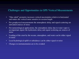
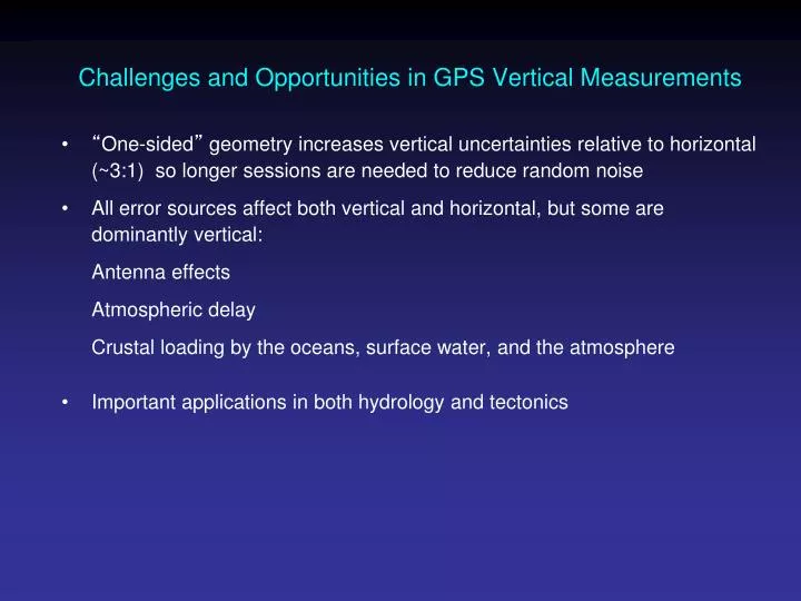
Challenges and Opportunities in GPS Vertical Measurements

1. Challenges and Opportunities in GPS Vertical Measurements • “One-sided” geometry increases vertical uncertainties relative to horizontal (~3:1) so longer sessions are needed to reduce random noise • All error sources affect both vertical and horizontal, but some are dominantly vertical: Antenna effects Atmospheric delay Crustal loading by the oceans, surface water, and the atmosphere • Important applications in both hydrology and tectonics

2. Time series for continuous station in (dry) eastern Oregon Vertical wrms 5.5 mm, higher than the best stations. Systematics may be atmospheric or hydrological loading, Local hydrolology, or Instrumental effects

3. Antenna Effects • Signal reflections in an antenna’s far field (multipathing) follow the laws of geometrical optics; period of oscillation depends on the distance to the reflector • Signal distortions in an antenna’s near field (phase center variations or PCVs) follow the laws of physical optics and are much more difficult to model

4. Antenna Ht 0.15 m 0.6 m Simple geometry for incidence of a direct and reflected signal: interference causes a phase shift 1 m Multipath contributions to observed phase for three different antenna heights [From Elosegui et al, 1995]

5. Left: Phase residuals versus elevation for Westford pillar, without (top) and with (bottom) microwave absorber. Right: Change in height estimate as a function of minimum elevation angle of observations; solid line is with the unmodified pillar, dashed with microwave absorber added [From Elosequi et al.,1995]

6. Top: PBO station near Lind, Washington. Bottom: BARD station CMBB at Columbia College, California (phtoto not available)

7. Antenna Phase Patterns

8. Modeling Antenna Phase-center Variations (PCVs) • Ground antennas • Relative calibrations by comparison with a ‘standard’ antenna (NGS, used by the IGS prior to November 2006) • Absolute calibrations with mechanical arm (GEO++) or anechoic chamber • May depend on elevation angle only or elevation and azimuth • Current models are radome-dependent • Errors for some antennas can be several cm in height estimates • Satellite antennas (absolute) • Estimated from global observations (T U Munich) • Differences with evolution of SV constellation mimic scale change Recommendation for GAMIT: Use latest IGS absolute ANTEX file with AZ/EL for ground antennas and ELEV (nadir angle) for SV antennas (MIT file augmented with NGS values for antennas missing from IGS)

9. Effect of the Neutral Atmosphere on GPS Measurements Slant delay = (Zenith Hydrostatic Delay) * (“Dry” Mapping Function) + (Zenith Wet Delay) * (Wet Mapping Function) • To recover the water vapor (ZWD) for meteorological studies, you must have a very accurate measure of the hydrostatic delay (ZHD) from a barometer at the site. • For height studies, a less accurate model for the ZHD is acceptable, but still important because the wet and dry mapping functions are different (see next slides) • The mapping functions used can also be important for low elevation angles • For both a priori ZHD and mapping functions, you have a choice in GAMIT of using values computed at 6-hr intervals from numerical weather models (VMF1 grids) or an analytical fit to 20-years of VMF1 values, GPT and GMF (defaults)

10. Percent difference (red) between hydrostatic and wet mapping functions for a high latitude (dav1) and mid-latitude site (nlib). Blue shows percentage of observations at each elevation angle. From Tregoning and Herring [2006].

11. Effect of error in a priori ZHD Difference between a) surface pressure derived from “standard” sea level pressure and the mean surface pressure derived from the GPT model. b) station heights using the two sources of a priori pressure.c) Relation between a priori pressure differences and height differences. Elevation-dependent weighting was used in the GPS analysis with a minimum elevation angle of 7 deg.

12. SShort-period Variations in Surface Pressure not Modeled by GPT Differences in GPS estimates of ZTD at Algonquin, Ny Alessund, Wettzell and Westford computed using static or observed surface pressure to derive the a priori. Height differences will be about twice as large. (Elevation-dependent weighting used).

13. Multipath and Water Vapor Can be Seen in the Phase Residuals

14. Annual Component of Vertical Loading Atmosphere (purple) 2-5 mm Snow/water (blue) 2-10 mm Nontidal ocean (red) 2-3 mm From Dong et al. J. Geophys. Res., 107, 2075, 2002

15. Atmospheric pressure loading near equator Vertical (a) and north (b) displacements from pressure loading at a site in South Africa. Bottom is power spectrum. Dominant signal is annual. From Petrov and Boy (2004)

16. Atmospheric pressure loading at mid-latitudes Vertical (a) and north (b) displacements from pressure loading at a site in Germany. Bottom is power spectrum. Dominant signal is short-period.

17. Spatial and temporal autocorrelation of atmospheric pressure loading From Petrov and Boy, J. Geophys. Res.,109, B03405, 2004

18. GAMIT Options for Modeling the Troposphere and Loading • For height studies, the most accurate models for a priori ZHD and mapping functions are the VMF1 grids computed from numerical weather models at 6-hr intervals. • For most applications it is sufficient to use the analytical models for a priori ZHD (GPT) and mapping functions (GMF) fit to 20 years of VMF1. • For meteorological studies, you need to use surface pressure measured at the site to compute the wet delay, but this can be applied after the data processing (sh_met_util), and it is sufficient to use GPT in the GAMIT processing • For height studies, atmospheric loading from numerical weather models (ATML grids) should also be applied. (ZHD and ATML are correlated, so don’t use one set of grids without the other)

19. Vertical Measurements over Short Baselines • Dominant errors are the antenna environment, hydrology, and water vapor (loading signals and atmospheric pressure have longer wavelengths) • Basellines less than a few km allow partial cancellation of water vapor as well • L1-only (or L1+L2) has less multipath noise than LC but ionospheric effects are typically 0.5-10 ppm, so LC may be better even for short baselines • Monumentation, environment, and setup are especially critical for sub-mm measurements Look at an example of measuring subsidence from pumping of an aquifer at 80-300 m) in the (dry) western US [ Burbey et al., J. Hydrology, 2006 ]

20. D=1640 D=1260 D= 620 Horizontal measurements 24-hr sessions, baselines 600-1600 m rms noise varies from 0.1 mm (shortest distance, driest days) to 0.5 mm ( VTnn are station names; R is distance from well; D distance from reference station ) Vertical measurements rms noise 0.6-3.0 mm [ Burbey et al., J. Hydrology, 2006 ] D=1640 D=1260 D= 620