Lecture 1 Density curves and the CLT

Lecture 1Density curves and the CLT Quantitative Methods Module I Gwilym Pryce g.pryce@socsci.gla.ac.uk

Notices: • Register • Feedback forms • Labs: • Who wants to do the afternoon lab? • Who wants to do the evening lab? • Class Reps and Staff Student committee. • Message: • those in Business taking the Master Class this week: come to seminar room 3 on the 3rd floor of the Business school at 10.00 on Wednesday? Thanks, Andy Furlong

Introduction: • In this lecture we introduce some statistical theory • This theory sometimes seems abstract for an applied quants course: • tempting just to use SPSS without properly learning statistical theory, • which is a very powerful statistical package • … but a little knowledge is a dangerous thing...

Aims & Objectives • Aim • the aim of this lecture is to introduce the concepts that under gird statistical inference • Objectives • by the end of this lecture students should be able to: • Understand what a density curve is • understand the principles that allow us to make inferences about the population from samples

Plan • 1. Review of Induction material • 2. Density curves & Symmetrical Distributions • 3. Normal Distribution • 4. Central Limit Theorem

1. Review of Induction material • 1.Measures of Central Tendency • 2. Measures of Spread • range, standard deviation • percentiles & outliers • Symmetric distributions • 3. Density curves • 4. Distribution of means from repeated samples = central limit theorem. • 5. Normal Distribution

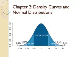
2. Density curves: idealised histograms (rescaled so that area sums to one)

Properties of a density curve • Vertical axis indicates relative frequency over values of the variable X • Entire area under the curve is 1 • The density curve can be described by an equation • Density curves for theoretical probability models have known properties

Area under density curves: • the area under a density curve that lies between two numbers = the proportion of the data that lies between these two numbers: • e.g. if area between two numbers x1 and x2 = 0.6, then this means 60% of xi lies between x1 and x2 • when the density curve is symmetrical, we make use of the fact that areas under the curve will also be symmetrical

Symmetrical Distributions Mean = median Areas of segments symmetrical 50% of sample < mean 50% of sample > mean Mean = median

Symmetrical Distributions • If 60% of sample falls between a and b, what % greater than b? • What’s the probability of randomly choosing an observation greater than b? 60% a b

What’s the probability of being less than 6ft tall? 20% height 6ft

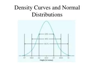
3. Normal distribution: 68% and 95% rules • Slide 10 of 13 of Christian’s.

Normal Curves are all related • Infinite number of poss. normal distributions • but they vary only by mean and S.D. • so they are all related -- just scaled versions of each other • a baseline normal distribution has been invented: • called the standard normal distribution • has zero mean and one standard deviation

b a c Standardise z zb zc za

Standard Normal Curve • we can standardise any observation from a normal distribution • I.e. show where it fits on the standard normal distribution by: • subtracting the mean from each value and dividing the result by the standard deviaiton. • This is called the z-score = standardised value of any normally distributed observation. Where m = population mean s = population S.D.

Areas under the standard normal curve between different z-scores are equal to areas between corresponding values on any normal distribution • Tables of areas have been calculated for each z-score, • so if you standardise your observation, you can find out the area above or below it. • But we saw earlier that areas under density functions correspond to probabilities: • so if you standardise your observation, you can find out the probability of other observations lying above or below it.

4. Distribution of means from repeated samples • We have looked at how to calculate the sample mean • What distribution of means do we get if we take repeated samples?

E.g. Suppose the distribution of income in the population looks like this:

Then suppose we ask a random sample of people what their income is. • This sample will probably have a similar distribution of income as the population • Positive skew: mean is “pulled-up” by the incomes of fat-cat, bourgeois capitalists. • Since the median is a “resistant measure”, the mean is greater than the median • Then suppose we take a second sample, and then a third; and then compute the mean income of each sample: • Sample 1: mean income = £20,500 • Sample 2: mean income = £18,006 • Sample 3: mean income = £21,230

As more samples are taken, normal distribution of mean emerges

Why the normal distribution is useful: • Even if a variable is not normally distributed, its sampling distribution of means will be normally distributed, provided n is large (I.e. > 30) • I.e. some samples will have a mean that is way out of line from population mean, but most will be reasonably close. • “Central Limit Theorem”

“The Central Limit Theorem is the fundamental sampling theorem. It is because of this theorem (and variations thereof), and not because of nature’s questionable tendency to normalcy, that the normal distribution plays such a key role in our work” (Bradley & South) • Why….?

The standard error of the mean... • When we are looking at the distribution of the sample mean, the standard deviation of this distribution is called the standard error of the mean • I.e. SE = standard deviation of the sampling distribution. • but we don’t usually know this • I.e. if we don’t know the population mean (I.e. mean of all possible sample means), we are unlikely to know the standard error of sample means • so what can we do?

CLT: What about Proportions? • What proportion of 10 catchers were female? • What happens if I repeat the experiment? • What would the distribution of sample proportions look like?

Editing syntax files: 1. Start with an asterix: • Use *blah blah blah. to put headings in syntax • anything after “ * ” is ignored by SPSS. • Important way of keeping your syntax files in order • e.g. *Descriptive Statistics on Income. *---------------------------------. 2. Forward slash and an asterix: • Use /*blah blah blah */to comment on lines • Anything between /* and */ is ignored by SPSS. • E.g. COMPUTE z = x + y. /*Compute total income*/

Lecture 1 Density curves and the CLT