Download
1 / 102
1.02k likes | 1.13k Views
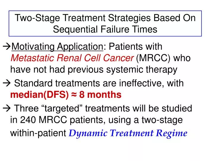
Two-Stage Treatment Strategies Based On Sequential Failure Times. Motivating Application : Patients with Metastatic Renal Cell Cancer (MRCC) who have not had previous systemic therapy Standard treatments are ineffective, with median(DFS) ≈ 8 months

E N D
Two-Stage Treatment Strategies Based On Sequential Failure Times • Motivating Application: Patients withMetastatic Renal Cell Cancer (MRCC) who have not had previous systemic therapy • Standard treatments are ineffective, with median(DFS) ≈ 8 months Three “targeted” treatments will be studied in 240 MRCC patients, using a two-stage within-patient Dynamic Treatment Regime
A Within-Patient Two-Stage Treatment Assignment Algorithm (Dynamic Treatment Regime) Stage1 At entry, randomize the patient among the stage 1 treatment pool {A1,…,Ak} Stage 2 If the 1st failure is disease worsening (progression of cancer) & not discontinuation, re-randomize the patient among a set of treatments {B1,…,Bn} not received initially “Switch-Away From a Loser”
Frontline Salvage Strategy ABC • B = (A, B) • C = (A, C) • A = (B, A) • C = (B, C) • A = (C, A) • B = (C, B)
Goal of the Renal Cancer Trial Select the two-stage strategy having the largest “average” time to second treatment failure (“overall failure time”) In the “null” case where all 6 strategies give the same overall failure time, each strategy is selected with probability 1/6
Outcomes T1 = Time to 1st treatment failure T2 = Time from 1st disease worsening to 2nd treatment failure T1 + T2 = Time of 2nd treatment failure
Unavoidable Complications Because disease is evaluated repeatedly (MRI, PET),either T1 or T1 + T2may be interval censored There may be a delay between 1st failure and start of stage 2 therapy T1 may affect T2 The failure rates may change over time (they increase for MRC)
Delay before start of 2nd stage rx Discontinuation Start of stage 2 rx
T2,1 = Time from 1st progression to 2nd treatment failure if it occurs during the delay interval before stage 2 therapy is begun T2,2 = Time from 1st progression to 2nd treatment failure if it occurs after stage 2 therapy has begun
A Parametric Model Weib(a,x) = Weibull distribution with meanm(a,x) = ea G(1+e-x), for real-valued a and x [ T1 | A ] ~ Weib(aA,xA) [ T2,1 | A,B, T1] ~ Exp{ gA+bA log(T1) } [ T2,2 | A,B, T1] ~ Weib( gA,B+bA log(T1), xA,B)
Establishing Priors q has 28 elements, but the 6 subvectors are qA,B= (n1,A, n2,A,B , aA , xA, gA, bA , aA,B , xA,B) Pr(Dis. Worsening)Reg. of T2 on T1 Weib pars of T1Weib pars of T2 The qA,B’s are exchangeable across the 6 strategies, so they have the same priors
Establishing Priors n1,A ,n2,A,B~ iid beta(0.80, 0.20) based on clinical experience aA , xA, gA, bA , aA,B , xA,B ~ indep. normal priors Prior means: We elicited percentiles of T1 and [ T2 | T1 = 8 mos], & applied the Thall-Cook (2004) least squares method to determine means Prior variances: We set var{exp(aA)} = var{exp(xA)} = var{exp(xA,B)} = 100 Assuming Pr(Disc. During delay period) = .02 E(mA,B) = 7.0 mos & sd(mA,B) = 12.9
Mean Overall Failure Time T = T1 + Y1,WT2 mA,B(q) = E{ T| (A,B)} = E(T1) + Pr(Y1,W =1)E(T2) Mean time to 1st failure Pr(1st failure is Disease Worsening) Mean time to 2nd failure
Criteria for Choosing a Best Strategy Mean{ mA,B(q) | data }: B-Weib-Mean 2. Median{ mA,B(q) | data }: B-Weib-Median 3. MLE of mA,B(q) under simple Exponential: F-Exp-MLE 4. MLE of mA,B(q) under full Weibull: F-Weib-MLE
A Tale of Four Designs Design 1 (February 21, 2006) N=240, accrual rate a = 12/month 20 month accrual + 18 mos addt’l FU Stage 1 pool = {A,B,C,D} 12 strategies (A,B), (A,C), (A,D), (B,A), (B,C), (B,D), (C,A), (C,B), (C,D), (D,A), (D,B), (D,C) Drop-out rate .20 between stages (240/12) x .80 = 16 patients per strategy
A Tale of Four Designs Design 2 (April 17, 2006) Following “advice” from CTEP, NCI : N = 240, a = 9/month (“more realistic”) Stage 1 pool = {A,B} (C, D not allowed as frontline) Stage 2 pool = {A,B,C,D} 6 strategies : (A,B), (A,C), (A,D), (B,A), (B,C), (B,D) (240/6) x .80 = 32 patients per strategy
A Tale of Four Designs An Interesting Property of Design 2 Stage 1 may be thought of as a conventional phase III trial comparing A vs B with size .05 and power .80 to detect a 50% increase in median(T1), from 8 to 12 months, embedded in the two-stage design However, the design does not aim to test hypotheses. It is a selection design.
A Tale of Four Designs Design 3 (January 3, 2007) CTEP was no longer interested, but several Pharmas were VERY interested N = 360, a = 12/month, 3 new treatments Stage 1 rx pool = Stage 2 rx pool = {a,s,t} 6 strategies (different from Design 2) : (a,s), (a,t), (s,a), (s,t), (t,a), (t,s) (360/6) x .80 = 48 patients per strategy
A Tale of Four Designs Design 4 (May 15, 2007) Question: Should a futility stopping rule be included, in case the accrual rate turns out to be lower than planned? Answer: Yes!! “Weeding” Rule: When 120 pats. are fully evaluated, stop accrual to strategy (a,b) if Pr{ m(a,b) < m(best) – 3 mos | data} > .90
A Tale of Four Designs Applying the Weeding Rule when 120 patients have been fully evaluated
Computer Simulations Simulation Scenarios specified in terms of z1(A) = median (T1 | A) and z2(A,B) = median { T2,2 | T1 = 8, (A,B) } Null values z1 = 8 and z2 = 3 z1 = 12 Good frontline z2 = 6 Good salvage z2 = 9 Very good salvage
Simulations: No Weeding Rule In terms of the probabilities of correctly selecting superior strategies, F-Weib-MLE ~ B-Weib-Median > B-Weib-Mean >> F-Exp-MLE
Sims With Weeding Rule • Correct selection probabilities are affected only very slightly • There is a shift of patients from inferior strategies to superior strategies – but this only becomes substantial with lower accrual rates
An Acute Leukemia Trial Comparing Two-Stage Treatment Strategies Thall, Sung and Estey, 2002 1) Each patient receives 1 or 2 courses of rx 2) Re-randomization for course 2 rx 3) Historical data are used to estimate non-treatment (“baseline”) model parameters 4) Interimly, the design drops inferior 2-stage strategies within subgroups
Trial Conduct Treatment Stage 1 : Randomize patients with probs. 1/3 each among the three course 1 treatments, balancing dynamically on patient covariates Treatment Stage 2 : Re-randomize patients whose course 1 treatment fails (patient is alive but disease is resistant to this chemotherapy) Weeding Out Inferior Strategies: Half-way through the trial, based on a trade-off-based utility of the probabilities of response and death, drop inferior treatment strategies within each prognostic subgroup
Treatments and Outcomes 0 = Standard treatment (Idarubicin + ara-C) 1, 2 = indices of the two experimental treatments Four two-course strategies were considered : (0,1), (0,2), (1,0), (2,0) Yk,c = I[Outcome k in course c] for k=R, D, F and c = 1,2 tj = treatment assigned in course j
A model for two-course treatment strategies pk1(s,Z) = Pr(Yk1 = 1 | t1=s, Z) pk2(s,t, Z) = Pr(Yk2 = 1 | t1=s, YF1=1, t2=t, Z) for k=R, D, F, treatments t1 and, t2 and baseline prognostic covariates Z = (Z1, …, Zq)
A GENERALIZED LOGISTIC MODEL Outcome k = R,D, strategy (s,t), covariates Z Course 1 Course 2
A GENERALIZED LOGISTIC MODEL TRT1 COV TRT1 x COV Outcome k = R,D, strategy (s,t), covariates Z Course 1 STRATEGY COURSE 2 Course 2
Overall 2-Stage Outcome Probabilities Outcome k = R,D, strategy (s,t), covariates Z A 2-Dimensional, Covariate-Adjusted Probability for Evaluating 2-Stage Strategies
Analysis of the Historical Data All parameters assumed to follow N(0,10) priors Covariates: [Age < 50 yrs], [1st CR Dur > 1 year] A hierarchy of models was considered BIC = Bayes Information Criterion used to assess fit
Simulation Study 1. The same p(qB| historical data) was used throughout 2. All others parameters assumed to follow N(0,10) priors 3. Maximum sample size = 96 patients, interim decisions to terminate subgroups made at 48 patients 4. 4000 replications for each of 4 clinical scenarios Results: In the presence of treatment-covariate interactions, the method reliably terminated inferior strategies early selected superior strategies within patient prognostic subgroups
Bayesian Geometric Approach to Treatment Comparison in Rapidly Fatal Diseases (Thall, Wooten and Shpall, 2005) The Problem In treatment of rapidly fatal diseases, Response (R) and Death Without Response are Competing Risks Example In cord blood transplantation (tx) for treatment of acute leukemia, Response = Engraftment =Recovery of neutrophil (white blood cell) count to a functional level (> 500 cells/mm3 blood)
TR + T2 if TR < T1 (Response Achieved) TD = T1 if TR > T1(Death w/o Response) TR Response T2 Treatment T1 Death
Given a initial time t* to achieve a Response, two parameters matter : p = Pr{ Respond by time t* } = Pr{ TR < min( t*,TD )} and m = E { TR | TR < TD }
Application: A randomized 60 patient trial tocompare two double cord blood tx methods, currently ongoing at MDACC “Expansion” = ex vivoselection and expansion of the cord blood cells Rx1 = Two unexpanded grafts Rx2 =One expanded + one unexpanded
Predictive covariate Z = Age, with 38 yrs. the physician’s reference value. For arm j = 1, 2, pj = Prj{ Engraft by day 42 | Z = 38 } = Prj { TR < min( 42,TD ) | Z = 38 } mj = mean time to engraftment = Ej (T | TR < TD , Z = 38)
If p1 = p2 = .70 but m1 = 14 days while m2 = 28 days, then method 1 is greatly superior to method 2. A statistical comparison based only on p1 and p2 , ignoring m1 and m2 , would be likely to conclude that p1 = p2 and make the false negative conclusion that the two methods do not differ. Why two parameters?
Defining the parameters (p, m) under a Competing Risks Model For k = R, D, 1 denote fk= pdf, Fk = cdf and = 1–Fk = survivor function of Tk
Technical Problem : How to compare the two treatments in terms of (p1, m1)versus(p2, m2)? Solution : Talk to your Physician ! Compared to the pair (p0, m0)of historical means with standard rx, elicit several equally desirabletarget pairs (p1*, m1*), . . . ,(pM*, mM*)that correspond to a “reference patient”Z*
Solution (continued) Use standard regression methods to fit a smooth, increasing curve D to the elicited pairs (p1*, m1*), . . . , (pM*, mM*),and identify the region QD ={(p, m) : p> p'and m<m'for some (p',m') on D} = The set of (p, m) pairsat least as desirable as a pair on the target contour
Denote the differences d12 = (p1- p2 , m1- m2)and djH = (pj- pH , mj- mH),for j = 1, 2. Evaluate & compare {d12 , d1H , d2H} a posteriori on the shifted set QD-(p0, m0) where (0,0) on QD-(p0, m0)corresponds to(p0 , m0)on QD.